Introduction
METROPOLIS2
METROPOLIS2 is an agent-based transport simulator.
Its main features are:
- 🚘 Mode choice (with an arbitrary number of modes, road vehicles are explicitly modeled)
- ⏱️ Continuous-time departure-time choice
- 🛣️ Deterministic route choice (for road vehicles)
- 👫 Agent based (each agent is an autonomous entity with its own characteristics and choices)
- 🚦 Modeling of road congestion (using speed-density functions and bottlenecks)
- ⏸️ Intermediary stops (with schedule preferences and stopping time at each intermediary point)
METROPOLIS2 is composed of
Metropolis-Core: a command line tool to run the transport simulations, written in Rust 🚀Pymetropolis: a command line tool to interact with METROPOLIS2’s input and output data, written in Python 🐍

What is this book?
This is the official documentation of METROPOLIS2, intended for anyone wanting to learn how to use the simulator and how it works.
It is divided in 2 parts: Pymetropolis (chapters 1 to 5) and Metropolis-Core (chapters 6 to 10).
Getting started
Pymetropolis is a Python command line tool that provides an automatic pipeline to generate, calibrate, run and analyze METROPOLIS2 simulation instances.
Pymetropolis can run many operations like:
- Importing a road network from OpenStreetMap data.
- Generating trips from an origin-destination matrix.
- Computing the walking distance of a set of trips.
- Calibrate some parameters to match mode shares from a travel survey.
- Generate the input files for the Metropolis-Core simulator.
- Run the Metropolis-Core simulator.
- Generate graphs from the results of the simulation.
Requirements ☑️
- Recent Python version (3.13+).
- Metropolis-Core
executables (
metropolis_cliandrouting_cli).
Installation 🔧
Pymetropolis’ releases are hosted on PyPI.
If you have pip installed (it is usually installed alongside Python), you can install Pymetropolis
by simply running:
pip install pymetropolis
To update Pymetropolis to a newer version, run:
pip install --upgrade pymetropolis
To check the version of pymetropolis that is installed on your system, run pymetropolis --version.
How it works 🤷♂️
Pymetropolis automates complex simulation workflows by executing a sequence of interdependent Steps. Each Step performs a specific computation and produces one or more MetroFiles (typically Parquet files) containing the results. Steps can also optionally consume MetroFiles as input, enabling flexible data processing.
Steps vary in complexity and functionality. They can:
- Import road networks from OpenStreetMap
- Generate trips from origin-destination matrices
- Compute walking distance for trips
- Run the Metropolis-Core simulator
- Build graphs from simulation results
Pymetropolis automatically determines the execution order of Steps and identifies which ones need re-running if changes occur.
A TOML configuration file defines the simulation instance, including:
- Which area is simulated?
- How the trips are generated?
- How the road network is imported?
- Which modes are available?
- What calibration is performed?
- Etc.
The Steps to execute are automatically derived from this configuration.
Once your configuration is ready, run:
pymetropolis my-config.toml
For large-scale simulations, execution may take hours or even days. If interrupted, Pymetropolis resumes from where it left off, skipping already completed Steps.
When you modify the configuration and re-run the command, Pymetropolis only executes the Steps affected by your changes (e.g., re-importing the road network is unnecessary if only the origin-destination matrix is updated).
Next steps 🧭
Explore practical examples and detailed documentation to get started:
- Case Studies: Step-by-step guides for running simulations, from toy networks to real-world, large-scale cities.
- Reference: Dive deeper into Pymetropolis components:
- Steps: Available processing steps.
- Parameters: All the parameters that can be used in the configuration.
- MetroFiles: Types of files generated and used by Pymetropolis.
Advanced use ⚙️
If you only want to see the Steps that need to be executed without actually running them, use the
--dry-run argument:
pymetropolis my-config.toml --dry-run
By default, Pymetropolis tries to execute all the Steps which are properly defined.
If you only require a specific Step to be executed, use the --step argument with the Step name:
pymetropolis my-config.toml --step PostprocessRoadNetworkStep
Getting help 🛟
Although Pymetropolis tries to be as reliable and universal as possible, various issues can arise due to the complexity of the process involved and the variety of datasets around the world. Many error messages have been included in the library to explain as clearly the issues that might have occurred.
If you found a bug or if there is a problem that you cannot fix, feel free to open an issue on the GitHub repository.
Concepts
Glossary
Zones
Pymetropolis uses zones to import origin-destination matrices and to analyze simulation results at different spatial levels.
Pymetropolis supports up to five hierarchical zone levels, labeled level1 to level5.
Each level can correspond to a specific administrative or geographic division, enabling multi-scale
analysis.
For France, the five zone levels align with the following administrative areas:
| Zone Level | Administrative Area | Description |
|---|---|---|
| level1 | Administrative Regions | Largest geographic division (NUTS1) |
| level2 | Départements | Intermediate administrative division |
| level3 | EPCI | Public Establishments of Intercommunal Cooperation |
| level4 | INSEE Municipalities | Cities and towns, including municipal districts |
| level5 | IRIS Zones | Smallest geographic units for detailed analysis |
Modes
car_driver
The agent is traveling by car. They are driver and presumably have no passenger.
- PCE = 1
- HOV lanes cannot be taken
- Fuel cost = 100%
car_driver_with_passengers
The agent is traveling by car. They are driver and have at least one passenger.
- PCE = 1
- HOV lanes cannot be taken
- Fuel cost = configurable
car_passenger
The agent is traveling by car but they are not driver.
- PCE = 0
- HOV lanes can be taken
- Fuel cost = configurable
car_ridesharing
The agent is traveling by car. There are m persons in the car. It is not known whether the agent is driver or passenger.
- PCE = 1 / m
- HOV lanes can be taken
- Fuel cost = 1 / m
public_transit
walking
bicycle
outside_option
Departure time
Warning
This page is a work-in-progress.
TODO: presentation of the different departure-time choice models in METROPOLIS2 + modeling considerations.
Setting departure_time_choice.mu to a very small value can lead to computational and convergence
issues, especially when agents are similar (similar preference parameters, similar origins and
destinations).
In METROPOLIS2, the utility function is modeled as a piecewise linear function.
It is thus not desirable for agents to choose the exact utility-maximizing departure time, as this
often falls on breakpoints, causing instability.
Therefore, using the Continuous Logit with a sufficiently large departure_time_choice.mu is
recommended in all scenarios, even when agents differ.
For further details, see Javaudin and de Palma (2024).
Javaudin, L., & de Palma, A. (2024). METROPOLIS2: Bridging theory and simulation in agent-based transport modeling. Technical report, THEMA, CY Cergy Paris Université.
Simulation convergence
- Definition of equilibrium and convergence
- What is a satisfying convergence?
- Which parameters influence convergence?
- How to choose the learning factor parameter?
- How to choose the correct number of iterations?
Modeling congestion
-
Bottlenecks
-
Spillback
-
Speed-density functions
-
Passenger Car Equivalent
-
Headway
Case studies
Bottleneck model
The simplest simulation that Pymetropolis can run:
- A single road with a bottleneck
- Identical agents with alpha-beta-gamma preferences
Circular City (coming soon)
- A configurable toy network representing a simplified city, with ring and radial roads.
- A gravity origin-destination matrix to easily simulate many trips.
Chambéry, France (coming soon)
- A real-case scenario for a medium-size French city.
- The road network is imported from OpenStreetMap data.
- The public-transit network is imported from GTFS data.
- A synthetic population is used to generate persons with a chain of activities.
- The simulation is calibrated to replicate TomTom and travel survey data.
Bottleneck (Toy model)
Estimated time to complete: 1 hour
The bottleneck model (Vickrey, 1969; Arnott, de Palma et Lindsey, 1990) is a foundational framework in transportation science, designed to analyze how traffic flow dynamics are constrained by capacity limitations at a single bottleneck within a road network.
This case study demonstrates how the bottleneck model with stochastic departure-time choice, as developed by de Palma, Ben-Akiva, Lefèvre, and Litinas (1983), can be replicated using METROPOLIS2. Note that, replicating the deterministic departure-time version remains challenging due to numerical limitations (see Javaudin and de Palma, 2024).
Theoretical framework
The bottleneck model features a single road with a free-flow travel time \(t^f\) and a bottleneck with capacity \(s\) (the maximum rate at which vehicles can cross the bottleneck).
\(N\) agents needs to cross the road and the bottleneck to travel from their origin to their destination. The number of agents is fixed and there is no alternative route which means that departure time is the only choice that matters.
Given a departure time \(t\), the deterministic utility of the agents is \[ v(t) = -\alpha T(t) - \beta [t^* - t - T(t)]^+ - \gamma [t + T(t) - t^*]^+ \tag{1} \] with
- \( \alpha \) the value of time,
- \(T\) the travel-time function,
- \( t^* \) the desired arrival time at destination,
- \( \beta \) the penalty for early arrivals,
- \( \gamma \) the penalty for late arrivals.
Using a Continuous Logit model, the probability that an agent chooses departure time \(t\) is given by \[ p(t) = \frac{ e^{v(t) / \mu} }{ \int_{t^0}^{t^1} e^{v(u) / \mu} d u } \tag{2} \] where \(\mu\) represents the randomness of departure-time choice and \([t^0, t^1]\) represents the period of possible departure times.
Preparation
Simulating the bottleneck model with Pymetropolis is straightforward: you first need to create a TOML configuration file that defines the model parameters and then you need to run Pymetropolis against this file.
Begin by creating a TOML file, such as config-bottleneck.toml, in your preferred directory.
This file will contain all the necessary settings for your simulation.
First, specify the directory where all simulation files will be stored using the
main_directory parameter.
main_directory = "bottleneck-sim/"
You can provide either an absolute path or a relative path for this directory.
Caution
If you use a relative path, it will be interpreted relative to the working directory from which you run Pymetropolis, which might differ from the directory where the configuration file is located.
To ensure your simulation results are reproducible, you can set a random seed using the
random_seed parameter.
random_seed = 123454321
If you omit this parameter, your results may vary slightly each time you run the simulation, even with the same configuration.
Supply side
The supply side of the bottleneck model represents the transport infrastructure available for agents to travel. In this model, the infrastructure consists of a single road, connecting a unique origin to a unique destination, featuring a bottleneck.
This single-road network can be conceptualized as a simplified grid network with one row and two
columns.
You can define this network in the configuration using the
GridNetworkStep.
[grid_network]
nb_rows = 1
nb_columns = 2
length = 1000
right_to_left = false
The road length is set to 1 000 meters (1 km). In the bottleneck model, the length only influences the free-flow travel time of the road, which also depends on the road speed (see below). In this model, the free-flow travel time only shifts departure times without affecting the equilibrium itself. For this reason, it is common in the literature to normalize it to zero. You can do so by setting the length to 0 meters.
The parameter right_to_left is set to false to
ensure the network consists of a single road from the left node (origin) to the right node
(destination).
If set to true, an additional road in the opposite direction would be created.
To complete the road configuration, you need to define the speed limit and bottleneck capacity.
This is done using steps
PostprocessRoadNetworkStep and
ExogenousCapacitiesStep.
Two parameters control this configuration:
road_network.default_speed_limit: Sets the speed limit on the road (in km/h). Here, it is set to 120 km/h, resulting in a 30-second free-flow travel time from origin to destination.road_network.capacities: Defines the bottleneck capacity (in vehicles per hour per lane). In this example, it is set to 16 000 vehicles per hour per lane, meaning a vehicle can cross the bottleneck every 0.24 seconds (3600 / 16000).
[road_network]
default_speed_limit = 120
capacities = 16000
Note
The bottleneck capacity of 16 000 vehicles per hour per lane is unrealistic (real-world lanes typically handle no more than one car per second, or 3 600 cars per hour). However, this toy model serves as a simplified representation of real-world scenarios. It could represent a network of roads connecting suburbs to a city center. Alternatively, it could model a multi-lane corridor (e.g., 8 lanes with a capacity of 2 000 each).
You can explicitly define the number of lanes using the
road_network.default_nb_lanesparameter. However, since the total capacity is the critical factor, it is often more straightforward to keep the number of lanes at 1 (the default) and setroad_network.capacitiesdirectly to the desired total capacity.
Tip
By default, METROPOLIS2 assumes a bottleneck at both the start and end of each road, limiting entry and exit flows. However, when all vehicles travel at the same speed, only the entry bottleneck matters. This is because vehicles reach the end of the road at the same rate they cross the entry bottleneck. In the bottleneck model, the location of the bottleneck does not affect the equilibrium so the default METROPOLIS2 behavior can be unchanged.
Demand side
The demand side of the model represents the agents (commuters) and their travel behavior. Each agent makes a single trip. The first step is to generate these trips.
You can use ODMatrixEachStep to generate a fixed number
of trips for each pair of nodes in the road network.
The number of trips per origin-destination pair is controlled by the
node_od_matrix.each parameter.
[node_od_matrix]
each = 10000
Tip
Pymetropolis automatically detects that the left node has no incoming edge and the right node has no outgoing edge. As a result, trips are only generated from the left node to the right node, not in the reverse direction.
Since no additional population details are specified, Pymetropolis assumes that each trip is made by a unique person. Therefore, it will automatically generate as many persons as trips, with standard characteristics.
Following the standard bottleneck model, it is initially assumed that agents can only travel by
car.
To specify the available modes, use the
mode_choice.modes parameter.
[mode_choice]
modes = ["car_driver"]
Preferences for each mode are configured in the modes.* tables.
For the car driver mode, the value of time (in euros per hour) is defined using the
modes.car_driver.alpha parameter.
This value represents a negative utility: larger values penalize more longer travel times.
[modes]
[modes.car_driver]
alpha = 10
Tip
In this documentation, utilities and costs are typically expressed in euros. However, you can use any currency or unit of your choice. You just need to ensure consistency across all values. For example, if one value is specified in dollars, all utility and cost values must also be in dollars.
The additional preference parameters of the bottleneck model (\( \beta \), \( \gamma \),
\( t^* \)) are not mode-specific and therefore not defined in the modes.car_driver table.
Instead, these parameters are configured in the departure_time.linear_schedule table.
“Linear schedule” refers here to a form of utility function that penalize linearly early and late
arrivals relative to a “desired arrival time” (\( t^* \)).
Parameters
departure_time.linear_schedule.beta
and
departure_time.linear_schedule.gamma
are both specified in euros per hour and represent negative utilities: higher values represent
greater penalties for delays.
The parameter
departure_time.linear_schedule.tstar
represent the desired arrival time, specified in HH:MM:SS value.
[departure_time.linear_schedule]
beta = 5
gamma = 7
tstar = 07:30:00
This configuration indicates that agents aim to arrive at 7:30 a.m., with a larger penalty applied for late arrivals compared to early arrivals.
The parameters specified so far fully specify the utility function (Equation 1). The next step is to define how agents choose their departure time, i.e., the optimization process they use to select a departure time based on their utility.
In METROPOLIS2, the Continuous Logit model is the recommended approach for departure-time choice. This model assumes that agents select their departure time based on probabilities derived from Equation (2). The Continous Logit introduces unobserved heterogeneity, ensuring that even identical agents do no choose the exact same departure time, which helps avoid convergence issues. For further details, see the page on departure-time choice in METROPOLIS.
To use a Continuous Logit model, set the
departure_time_choice.model parameter
to "ContinuousLogit".
The
departure_time_choice.mu parameter controls
the level of randomness in the choice: smaller values make agents choose departure times closer
to the utility-maximizing value; larger values introduce more randomness in their choice.
[departure_time_choice]
model = "ContinuousLogit"
mu = 1
Simulation
Before running the simulation, a few final parameters must be configured in the simulation table.
First, the simulation.period parameter defines
the time window of the simulation as a list of two elements: the start time and the end time.
This period constrains when agents can depart, though some trips may finish after the end time.
The period also determines the time window during which road-level travel times are recorded.
Travel times are stored as piecewise linear functions, with the time between breakpoints controlled
by the simulation.recording_interval
parameter.
For the bottleneck simulation, it is recommended to set a one-hour period (e.g., from 7 a.m. to 8 a.m.) and to use a small recording interval (e.g., 60 seconds or less) to ensure that agents have precise travel time information when choosing their departure time.
Note
Setting the simulation period to one hour is a form of normalization. If you double the period, recording interval, number of agents, and departure-time mu, then the results will remain qualitatively similar.
Also, if you shift both the simulation period and the desired arrival time earlier or later by the same duration, then the departure and arrival times of the agents will shift accordingly.
Finally, two parameters are chosen to ensure the simulation converges satisfactorily:
simulation.learning_factorcontrols how quickly agents learns about travel times, a value of 0.1 is recommended;simulation.nb_iterationsdetermines the number of iterations the simulation runs, a value of 200 is typically sufficient here.
[simulation]
period = [07:00:00, 08:00:00]
recording_interval = 60
learning_factor = 0.1
nb_iterations = 200
Tip
For bottleneck simulations with a higher ratio of agents to bottleneck capacity, consider decreasing the learning factor or increasing the number of iterations.
For more details on simulation convergence, refer to the relevant page.
Also ensure that you have downloaded the last version of
Metropolis-Core and set
the metropolis_core.exec_path parameter to
point to the metropolis_cli executable.
By convention, the executable is typically placed in an execs/ directory within the directory
where Pymetropolis is executed.
[metropolis_core]
exec_path = "execs/metropolis_cli"
Note
For Windows user, you do not need to add the
".exe"extension tometropolis_cliinexec_path. It is actually recommended not to do so, so that your configuration can be shared easily with MacOS and Linux users.
Running
Once your configuration file is ready, you can execute Pymetropolis directly from the terminal.
Simply run the pymetropolis command, specifying the path to your configuration file as an
argument.
Optionally, before running the full simulation, you can check what Pymetropolis is planning to do by
using the --dry-run option.
This will check for typos or issues and display the list of steps that will be executed:
pymetropolis config-bottleneck.toml --dry-run
If there everything is correctly configured, you should see an output similar to this.
1. WriteMetroParametersStep
2. GridNetworkStep
3. PostprocessRoadNetworkStep
4. AllRoadDistancesStep
5. ODMatrixEachStep
6. CarShortestDistancesStep
7. ExogenousCapacitiesStep
8. EdgesFreeFlowTravelTimesStep
9. AllFreeFlowTravelTimesStep
10. CarFreeFlowDistancesStep
11. GenericPopulationStep
12. WriteMetroEdgesStep
13. WriteMetroVehicleTypesStep
14. CarDriverPreferencesStep
15. LinearScheduleStep
16. WriteMetroAgentsStep
17. HomogeneousTstarStep
18. WriteMetroTripsStep
19. UniformDrawsStep
20. WriteMetroAlternativesStep
21. RunSimulationStep
22. IterationResultsStep
23. ConvergencePlotStep
24. RoadNetworkCongestionFunctionPlotsStep
25. TripResultsStep
26. TripDepartureTimeDistributionStep
If the list of steps looks correct, you can proceed with the actual simulation by removing the
--dry-run option.
pymetropolis config-bottleneck.toml
The simulation should complete in about one minute.
Convergence
Before diving into the results, the first step is to verify whether the simulation has converged satisfactorily. If the convergence is poor, further analysis may not be meaningful, and you may need to adjust the number of iterations or the learning factor (See Simulation convergence).
Pymetropolis automatically generates convergence graphs in the results/graphs/ directory
(located within the main_directory you specified).
These graphs are prefixed with convergence_.
For the bottleneck simulation, you can focus on these graphs:
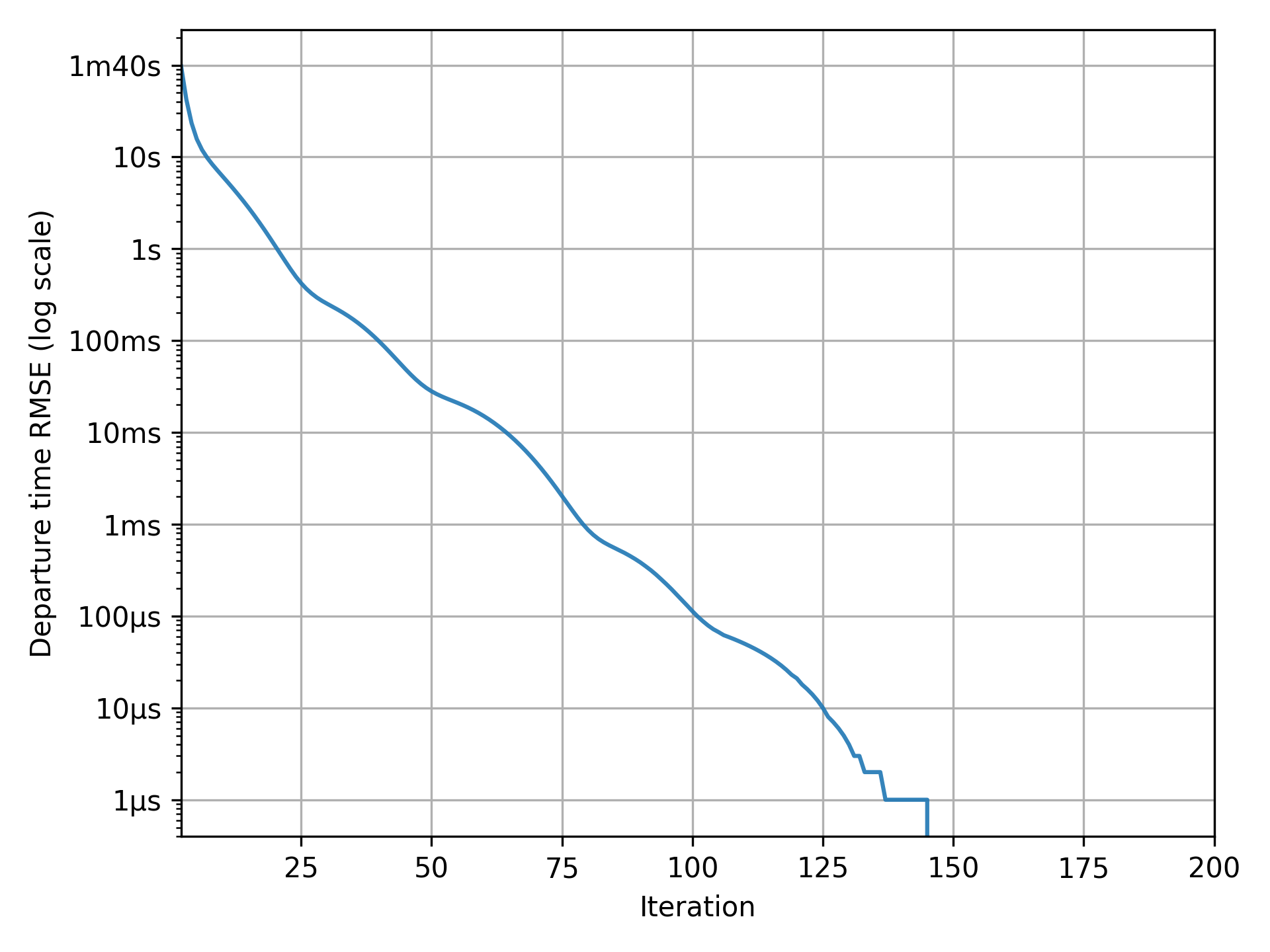
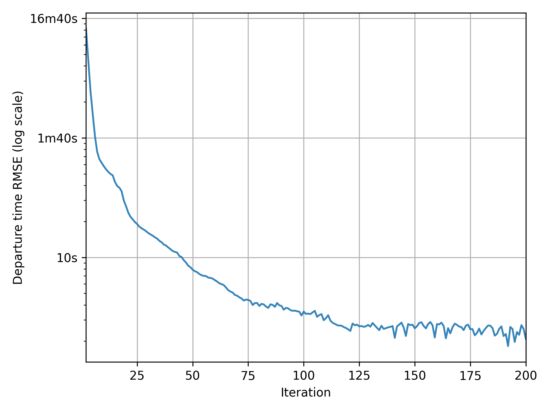
convergence_tour_departure_time.pngshows by how much departure times vary over iterations;convergence_simulated_road_travel_times.pngshows by how much the simulated travel-time function differs from the expected travel-time function over iterations.
If your graphs match the examples below, with the indicator consistently at zero in the final iterations, the simulation has perfectly converged and results are reliable for analysis.

Note
At each iteration of METROPOLIS2, all agents choose their preferred departure time, across the entire possible departure-time period, based on the current expected travel-time function. If the simulated travel-time function matches the expected travel-time function, it means that agents made optimal choices: they accurately anticipated travel conditions and have no reason to change their departure time. Therefore, when departure times and travel times are unchanged between iterations, the simulation has effectively reached an equilibrium.
Tip
In this example, the simulation achieves perfect convergence. However, in more complex scenarios, perfect convergence may not always be attainable. Instead, ensure that the convergence indicators remain consistently low in the final iterations. This suggests that the simulation approximate an equilibrium, even if minor fluctuations persist. Such level of stability is often sufficient for meaningful analysis.
Results
Pymetropolis generates a variety of output files that you can use to analyze the simulation results. The most relevant files for the bottleneck simulation are:
results/iteration_results.parquetgives aggregate results across all iterations;results/trip_results.parquetgives trip-level results, including departure times, arrival times, utilities.
Feel free to explore these files to generate your own tables and graphs.
Pymetropolis also produces graphs to visualize key aspects of the simulation:
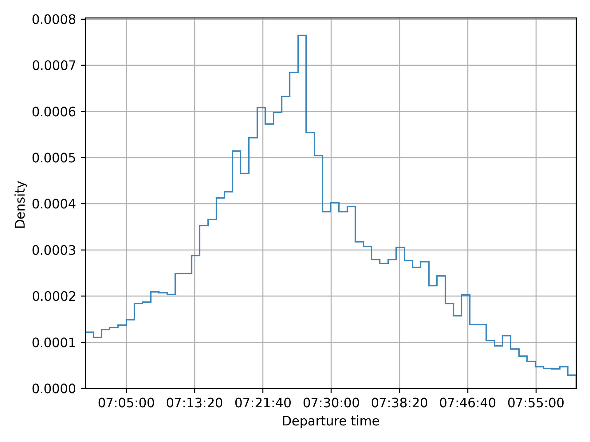
results/graphs/trip_departure_time_distribution.pngfor the distribution of departure times;results/graphs/network_congestion_function_expected.pngfor the congestion function on the road.

For additional graphs and a comparison with analytical results, refer to Javaudin and de Palma (2024).
Extensions
Elastic demand
A simple way to extend the bottleneck model is to incorporate elastic demand by giving agents an alternative to traveling by car. This alternative could represent options like using public transit or choosing not to travel at all.
In Pymetropolis, you can model such an alternative using the "outside_option" mode.
This mode provides a constant cost (or utility) alternative to the agents, without modeling
departure times or travel times.
The modes.outside_option.constant
parameter defines the constant cost associated to the outside option.
Based on the previous simulation results, where agents’ surplus is around 7.25, you can set the
outside option’s utility to 5 (i.e., its cost to -5) to ensure it remains less attractive than
driving.
[modes.outside_option]
constant = -5
Caution
The
[modes.outside_option]table must be nested within the[modes]section. If you are unsure about the syntax, refer to the TOML documentation or the complete configuration example below for guidance.
Adding the outside option introduces a new decision for agents: choosing between driving or not.
You need to specify how agents choose between these two options, using the
mode_choice.model parameter.
A standard approach is to use a Logit model, which allows agents to make probabilistic choices
based on the utility of each option.
Configure this by updating the [mode_choice] table in your configuration, setting
mode_choice.model to "Logit".
[mode_choice]
modes = ["car_driver", "outside_option"]
model = "Logit"
mu = 1
The mode_choice.mu parameter controls the level of
randomness in the choice: smaller values make agents more likely to choose the
utility-maximizing option; larger values introduce more randomness in their decision.
Also observe that you need to include "outside_option" in the list of modes available to the
agents.
Distributed parameters
So far, the simulated agents were identical: they shared the same origin, destination, value of time, schedule-delay penalties, and desired arrival time. Crucially, some form of heterogeneity was introduced through the Continous Logit model (for departure-time choice) and the Logit model (for mode choice). This heterogeneity is essential to prevent all agents from choosing the same departure time, which would result in unrealistic congestion patterns.
You can introduce additional variability by defining preference parameters, such as
modes.car_driver.alpha or departure_time.linear_schedule.beta, as distributions rather than
fixed values.
For example, to model the desired arrival time as a Normal distribution with a mean of 07:30:00 and
a standard deviation of 10 minutes (600 seconds), you can use the following configuration.
tstar = { mean = 07:30:00, std = 600, distribution = "Normal" }
The same syntax can be applied to any preference parameter that supports distributions. For more details on the syntax and the available distributions, refer to the Parameters page.
Complete configuration
main_directory = "bottleneck-sim/"

random_seed = 123454321

[grid_network]
nb_rows = 1
nb_columns = 2
length = 1000
right_to_left = false

[road_network]
default_speed_limit = 120
capacities = 16_000

[node_od_matrix]
each = 10_000

[mode_choice]
modes = ["car_driver"]
# Uncomment to add the outside option alternative.
#modes = ["car_driver", "outside_option"]
#model = "Logit"
#mu = 1

[modes]
[modes.car_driver]
alpha = 10

# Uncomment to add the outside option alternative.
#[modes.outside_option]
#constant = -5

[departure_time_choice]
model = "ContinuousLogit"
mu = 1

[departure_time.linear_schedule]
beta = 5
gamma = 7
# Constant tstar over agents.
tstar = 07:30:00
# Normally distributed tstar over agents.
#tstar = { mean = 07:30:00, std = 600, distribution = "Normal" }

[simulation]
period = [07:00:00, 08:00:00]
recording_interval = 60
learning_factor = 0.1
nb_iterations = 200

[metropolis_core]
exec_path = "execs/metropolis_cli"
References
Arnott, R., de Palma, A., & Lindsey, R. (1990). Economics of a bottleneck. Journal of urban economics, 27(1), 111-130.
de Palma, A., Ben-Akiva, M., Lefevre, C., & Litinas, N. (1983). Stochastic equilibrium model of peak period traffic congestion. Transportation Science, 17(4), 430-453.
Javaudin, L., & de Palma, A. (2024). METROPOLIS2: Bridging theory and simulation in agent-based transport modeling. Technical report, THEMA, CY Cergy Paris Université.
Vickrey, W. S. (1969). Congestion theory and transport investment. The American economic review, 59(2), 251-260.
Circular City (Toy model)
Estimated time to complete: 2 hours
This case study presents a toy model designed to be both simple and feature-rich:
- Quick to run: Executes in just a few minutes.
- Concise configuration: Requires only a single TOML file (~100 lines).
- Comprehensive: Incorporates most of METROPOLIS2’s core features, including mode choice, departure-time choice, route choice, fuel consumption, spillback effects, and ridesharing.
The model simulates an imaginary circular city, featuring ring roads (circular roads) and radial roads (arterial roads).
This structure is inspired by the foundational work of de Palma, Kilani, and Lindsey (2005), though it is not an exact replication. Instead, it offers a modern adaptation tailored for METROPOLIS2.
Preparation
As for the Bottleneck case study, begin by creating a TOML configuration file
(e.g., config-circular-city.toml) in your preferred directory.
This file serves as the foundation for your simulation.
Start by defining the main_directory and
random_seed parameters in your configuration file.
The main_directory specifies where all simulation outputs will be saved, while the random_seed
ensures your results are reproducible.
# config-circular-city.toml
main_directory = "circular-city/"

random_seed = 123454321
Supply side
The Circular City model uses the CircularNetworkStep
to create a customizable road network composed of ring roads and radial roads.
The nb_radials parameter defines the
number of directions for radial roads:
nb_radials = 4: creates radial roads in the North, East, South, and West directions;nb_radials = 8: adds Northeast, Northwest, Southeast, and Southwest directions;nb_radials = n: n roads are automatically generated starting from the East direction and are evenly spaced around the circle.
Parameter nb_rings controls the number of
concentric rings in the city and parameter
radius defines the distance between rings
(in meters).
If radius is a single value, for example radius = 2000, each ring is space 2 km apart from the
city center.
If radius is a list, for example radius = [1000, 1500] (with nb_rings = 2), the first ring is
1 km from the center and the second is 1.5 km from the center (500 m apart).
Nodes are automatically created at the intersection of each ring and radial road.
For more details, including how node and edge ids are generated, refer to the
CircularNetworkStep documentation.
For the same topological network as in de Palma et al. (2005), use the following configuration. Feel free to tweak it to your liking!
[circular_network]
nb_radials = 8
nb_rings = 4
radius = 4000
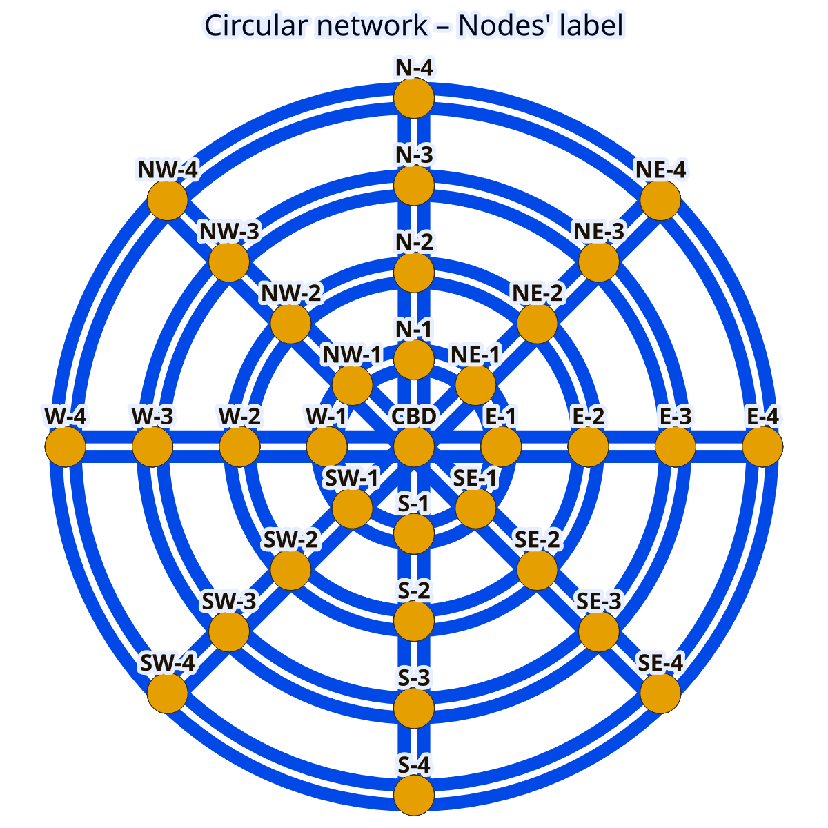
Figure 1. Circular network with node labels.
File used: edges_raw.geo.parquet
Tip
If you are more into American-style cities, consider creating a grid network instead.
To finalize the Circular City network configuration, you need to define the speed limits, number of
lanes and bottleneck capacities.
This is done using
PostprocessRoadNetworkStep and
ExogenousCapacitiesStep, similar to the
Bottleneck case study.
The key parameters are:
road_network.default_speed_limitsets the speed limit (in km/h);road_network.default_nb_lanesdefines the number of lanes (in one direction);road_network.capacitiesspecifies the bottleneck capacity (in vehicles per hour per lane).

Figure 2. Circular network with edges’ road types.
Edges with the same color share the same road type.
File used: edges_raw.geo.parquet
The values can be specified per road type (see map) by providing a TOML table with the road-type labels as keys. To replicate the values from de Palma et al. (2005), use the following configuration.
[road_network]
[road_network.default_speed_limit]
"Radial 1" = 50
"Radial 2" = 50
"Radial 3" = 50
"Radial 4" = 50
"Ring 1" = 50
"Ring 2" = 70
"Ring 3" = 70
"Ring 4" = 70

[road_network.default_nb_lanes]
"Radial 1" = 2
"Radial 2" = 2
"Radial 3" = 2
"Radial 4" = 2
"Ring 1" = 1
"Ring 2" = 1
"Ring 3" = 1
"Ring 4" = 1

[road_network.capacities]
"Radial 1" = 1500
"Radial 2" = 2000
"Radial 3" = 2000
"Radial 4" = 2000
"Ring 1" = 2000
"Ring 2" = 2000
"Ring 3" = 2000
"Ring 4" = 2000
Demand side
To simulate trips in the Circular City model, you can use an origin-destination matrix, where road-network nodes serve as origins and destinations.
In real-world scenarios, the number of trips between two nodes typically decreases with distance.
The GravityODMatrixStep models this effect by
assuming that the number of trips between nodes decays exponentially with distance.
The key parameters for this step are defined below.
trips_per_nodedefines the total number of trips originating from each node.exponential_decaycontrols how quickly the number of trips decreases with distance. Withexponential_decay = 0, trips originating from a node are uniformly distributed across all destinations. With higher values, more trips are concentrated toward closer destinations.
[gravity_od_matrix]
trips_per_node = 8000
exponential_decay = 0.07

Figure 3. Flows originating from node “NE-2”.
Files used: road_origin_destination_matrix.geo.parquet,
edges_raw.geo.parquet
Tip
If you want different number of trips originating from each node, you can define
trips_per_nodeas a distribution. For example:
trips_per_node = { mean = 8000, std = 1000, distribution = "Normal" }
Tip
For full control over trip generation, you can create your own origin-destination matrix and use it with the
CustomODMatrixStep.
To align with de Palma et al. (2005), you can configure agents to choose between car and public transit using a Logit model. This setup allows agents to make probabilistic choices based on the utility of each mode.
[mode_choice]
modes = ["car_driver", "public_transit"]
model = "Logit"
mu = 1
The parameters are defined as follow.
modeslists the available travel modes.modeluses the Logit model for mode choice.mucontrols the randomness in mode select. Lower values means that agents are more likely to choose the maximum-utility mode.
Tip
For more advanced scenarios, you can include ridesharing as an additional mode. This extension is explored further in the Extensions section.
Preferences for each mode are defined in the modes.* tables.
Each mode includes two parameters.
alpharepresents the value of time (in euros per hour).constantrepresents a fixed cost associated with choosing the mode.
[modes]
[modes.car_driver]
constant = 0
alpha = 10

[modes.public_transit]
constant = 2.0
alpha = 15.0
road_network_speed = 40
The parameter
road_network_speed simplifies
public-transit travel time calculation by assuming a constant speed on the road network, avoiding
the need to define a separate public-transit network.
A value of 40 km/h matches the assumption from de Palma et al. (2005).
As in the Bottleneck case study, you can include schedule-delay penalties in the
utility function using the departure_time.linear_schedule table.
These penalties influence agents’ departure-time choice based on their desired arrival time.
betadefines the penalty for early arrivals (in euros per hour).gammadefines the penalty for late arrivals (in euros per hour).tstarrepresent the desired arrival time at destination, specified inHH:MM:SSformat.
[departure_time.linear_schedule]
beta = 6
gamma = 25
tstar = { mean = 08:00:00, std = 1800, distribution = "Uniform" }
This configuration means that agents have a desired arrival time uniformly distributed between
07:30:00 and 08:30:00.
Late arrivals incur a higher penalty (25 euros per hour) compared to early arrivals (6 euros per
hour).
To model how agents choose their departure time, it is recommended using the Continuous Logit model, which aligns with the approach in de Palma et al. (2005).
Set departure_time_choice.model
to "ContinuousLogit" and use
departure_time_choice.mu to control
the randomness in agents’ choices: smaller values make agents choose departure times closer
to the utility-maximizing value; larger values introduce more randomness in their choice.
[departure_time_choice]
model = "ContinuousLogit"
mu = 1
Simulation
Before running the simulation, configure the final parameters in the simulation table.
[simulation]
period = [06:00:00, 10:00:00]
recording_interval = 300
learning_factor = 0.005
nb_iterations = 200
The simulation.period parameter defines
the time window of the simulation, specified as a list of start and end times.
This period constrains when agents can depart.
For this simulation, focused on the morning peak period (with desired arrival times between 07:30 and 08:30), a period from 6 a.m. to 10 a.m. provides a sufficiently wide window for all agents to depart and reach their destinations.
Tip
If you notice a peak of departures at the very start or end of the simulation period, it may indicate that the period is too narrow. Extend the window to allow agents to choose departure times that align better with their desired arrival times.
The simulation.recording_interval
parameter controls the time between breakpoints in the piecewise linear functions used to store
travel times.
A value of 300 seconds (5 minutes) offers a good balance between simulation speed and accuracy in
travel-time functions.
To ensure the simulation converges satisfactorily, two key parameters are defined.
simulation.learning_factorcontrols how quickly agents learns about travel times. A value of 0.005 is recommended for this simulation.simulation.nb_iterationsdetermines the number of iterations the simulation runs. A value of 200 is typically sufficient.
Tip
For simulations with higher congestion, consider decreasing the learning factor or increasing the number of iterations to improve the convergence quality.
For more details on simulation convergence, refer to the relevant page.
Before running your simulation, ensure you have downloaded the last version of
Metropolis-Core and configured the
metropolis_core.exec_path parameter to
point to the metropolis_cli executable.
By convention, the executable is typically placed in an execs/ directory within the directory
where Pymetropolis is executed.
[metropolis_core]
exec_path = "execs/metropolis_cli"
Running
Once your configuration file is ready, you can execute Pymetropolis directly from the terminal.
Simply run the pymetropolis command, specifying the path to your configuration file as an
argument.
Optionally, before running the full simulation, you can check what Pymetropolis is planning to do by
using the --dry-run option.
This will check for typos or issues and display the list of steps that will be executed:
pymetropolis config-circular-city.toml --dry-run
If there everything is correctly configured, you should see an output similar to this.
1. WriteMetroParametersStep
2. CircularNetworkStep
3. PostprocessRoadNetworkStep
4. AllRoadDistancesStep
5. ExogenousCapacitiesStep
6. EdgesFreeFlowTravelTimesStep
7. AllFreeFlowTravelTimesStep
8. GravityODMatrixStep
9. CarFreeFlowDistancesStep
10. CarShortestDistancesStep
11. GenericPopulationStep
12. WriteMetroEdgesStep
13. WriteMetroVehicleTypesStep
14. CarDriverPreferencesStep
15. PublicTransitPreferencesStep
16. PublicTransitTravelTimesFromRoadDistancesStep
17. RoadODMatrixStep
18. LinearScheduleStep
19. HomogeneousTstarStep
20. WriteMetroTripsStep
21. UniformDrawsStep
22. WriteMetroAgentsStep
23. WriteMetroAlternativesStep
24. RunSimulationStep
25. IterationResultsStep
26. ConvergencePlotStep
27. RoadNetworkCongestionFunctionPlotsStep
28. TripResultsStep
29. TripDepartureTimeDistributionStep
If the list of steps looks correct, you can proceed with the actual simulation by removing the
--dry-run option.
pymetropolis config-circular-city.toml
The simulation should complete in about 20 minutes.
Convergence
Before diving into the results, the first step is to verify whether the simulation has converged satisfactorily. If the convergence is poor, further analysis may not be meaningful, and you may need to adjust the number of iterations or the learning factor (See Simulation convergence).
Pymetropolis automatically generates convergence graphs in the results/graphs/ directory (located
within the main_directory you specified).
These graphs are prefixed with convergence_ and fall into two main categories.
- Graphs with an indicator representing a change from one iteration to another.
The indicator should be close to zero in the final iterations.
Example graphs:
convergence_tour_departure_time.png: shifts in departure times,convergence_route_length_diff.png: shifts in route selected,convergence_simulated_road_travel_times.png: changes in road-level travel times.
- Graphs with an indicator representing an aggregate measure.
The indicator should stabilize to an equilibrium value in the final iterations.
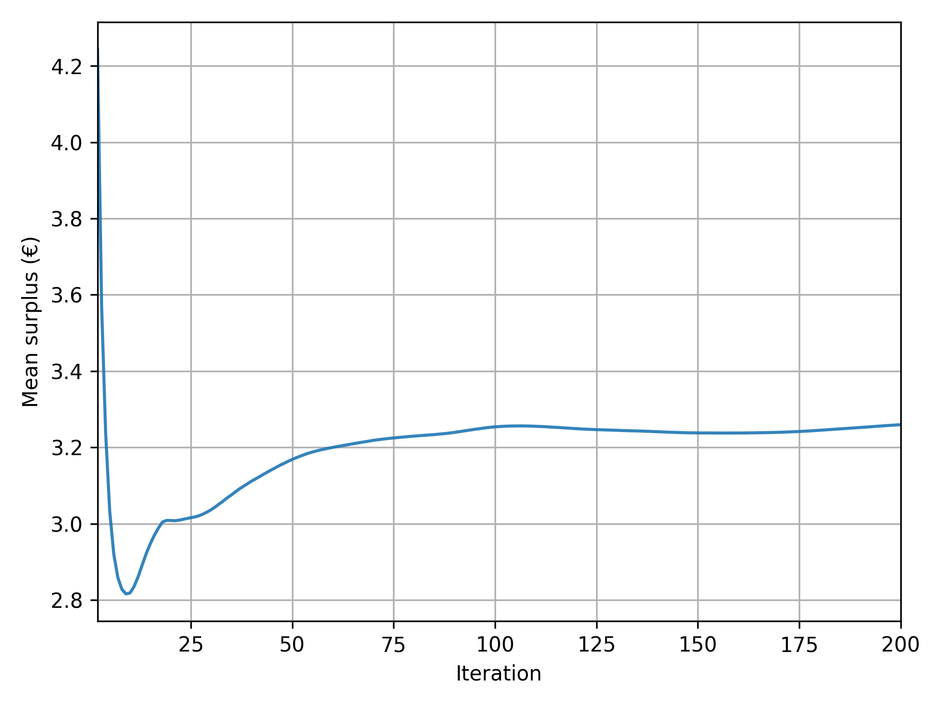
Example graphs:
convergence_mean_surplus.png: mean surplus,convergence_road_trips_share.png: share of road trips.
Results
Pymetropolis generates a variety of output files that you can use to analyze the simulation results. Some of the most relevant files are:
results/iteration_results.parquetgives aggregate results across all iterations;results/trip_results.parquetgives trip-level results, including departure times, arrival times, utilities.
Feel free to explore these files to generate your own tables and graphs.
Pymetropolis also produces graphs to visualize key aspects of the simulation:
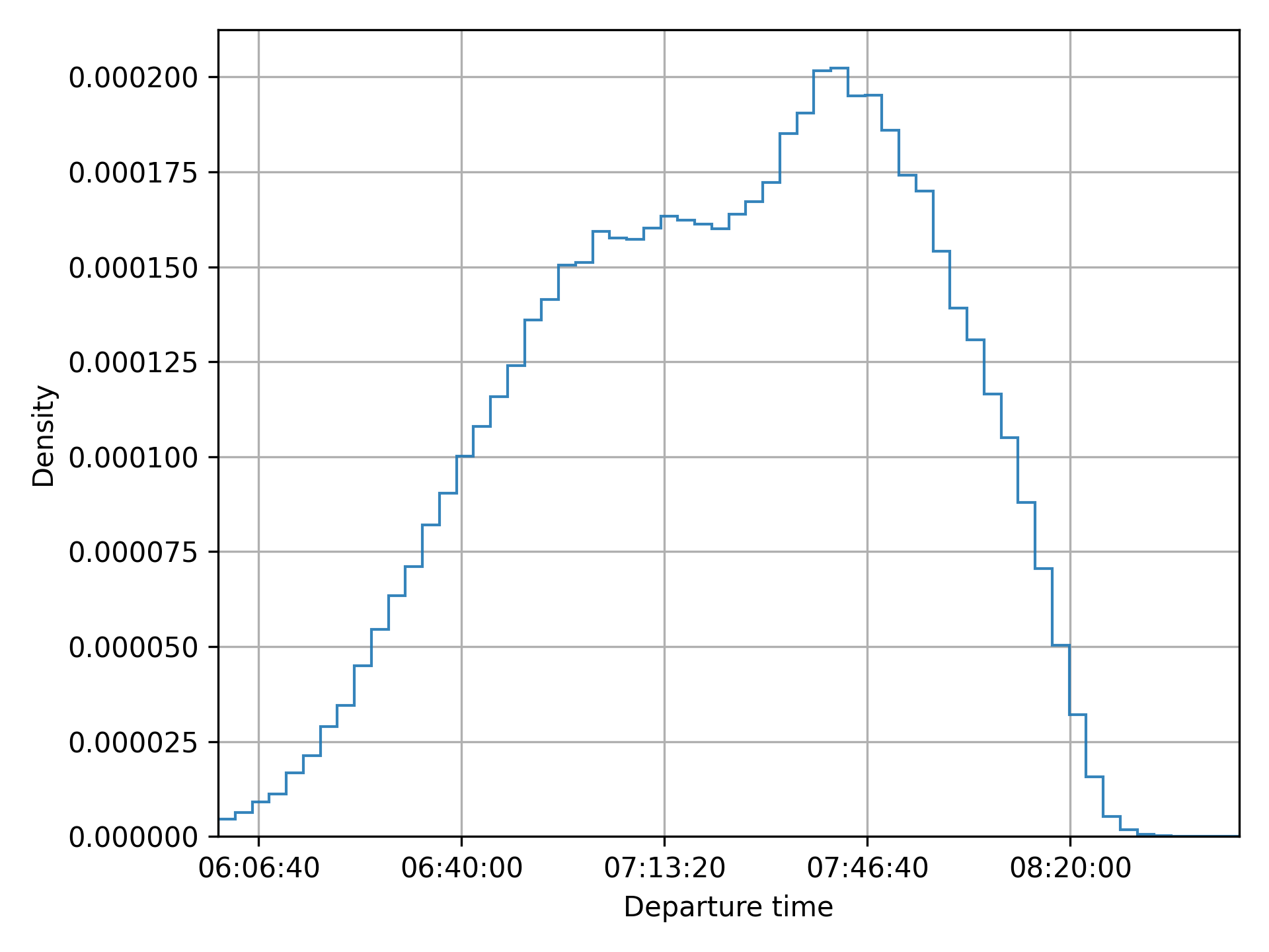
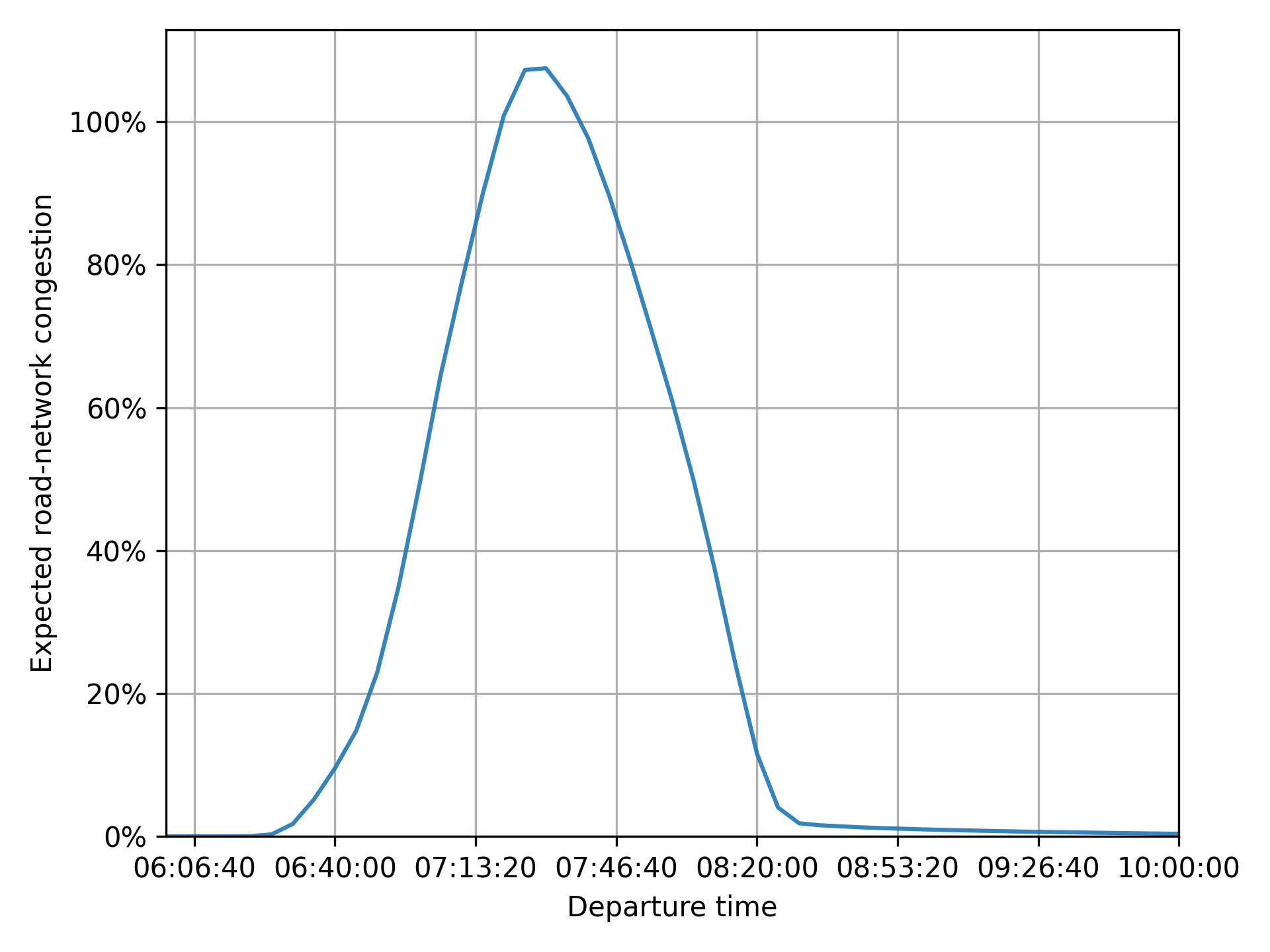
results/graphs/trip_departure_time_distribution.pngfor the distribution of departure times;results/graphs/network_congestion_function_expected.pngfor the congestion function on the road.
Complete configuration
main_directory = "circular-city/"

random_seed = 123454321

[circular_network]
nb_radials = 8
nb_rings = 4
radius = 4000

[road_network]
[road_network.default_speed_limit]
"Radial 1" = 50
"Radial 2" = 70
"Radial 3" = 70
"Radial 4" = 70
"Ring 1" = 50
"Ring 2" = 50
"Ring 3" = 50
"Ring 4" = 50

[road_network.default_nb_lanes]
"Radial 1" = 2
"Radial 2" = 2
"Radial 3" = 2
"Radial 4" = 2
"Ring 1" = 1
"Ring 2" = 1
"Ring 3" = 1
"Ring 4" = 1

[road_network.capacities]
"Radial 1" = 1500
"Radial 2" = 2000
"Radial 3" = 2000
"Radial 4" = 2000
"Ring 1" = 2000
"Ring 2" = 2000
"Ring 3" = 2000
"Ring 4" = 2000

[gravity_od_matrix]
exponential_decay = 0.07
trips_per_node = 8000

[mode_choice]
modes = ["car_driver", "public_transit"]
model = "Logit"
mu = 1

[modes]
[modes.car_driver]
constant = 0
alpha = 10

[modes.public_transit]
constant = 2
alpha = 15
road_network_speed = 40

[departure_time_choice]
model = "ContinuousLogit"
mu = 1

[departure_time.linear_schedule]
beta = 6
gamma = 25
tstar = { mean = 08:00:00, std = 1800, distribution = "Uniform" }

[simulation]
period = [06:00:00, 10:00:00]
recording_interval = 300
learning_factor = 0.005
nb_iterations = 200

[metropolis_core]
exec_path = "execs/metropolis_cli"
Extensions
Introducing ridesharing
In the current setup, agents traveling by car are assumed to be driving alone, with each agent generating congestion equivalent to a single car. However, in reality, people with similar origins and destinations often share rides to save on costs like fuel.
METROPOLIS2 proposes the "car_ridesharing" mode to model ridesharing.
This mode represents agents traveling by car with others, without distinguishing between drivers
and passengers.
To include this mode as an option for the agents, update the
mode_choice.modes parameter.
[mode_choice]
modes = ["car_driver", "car_ridesharing", "public_transit"]
Note
The
"car_ridesharing"mode is a basic representation of ridesharing in METROPOLIS2:
- It does not explicitly model the matching between drivers and passengers.
- It does not guarantee that agents choosing ridesharing have a compatible partner with the same origin, destination, and departure time.
- It does not account for detours drivers might take to pick up or drop off passengers.
For advanced ridesharing modeling in METROPOLIS2, including matching, refer to Ghoslya et al. (2025).
You can define preferences for the "car_ridesharing" mode different from the ones for
"car_driver".
constantrepresents the fixed cost of ridesharing (e.g., difficulty finding a match, detours, waiting time).alpharepresents the value of time (which can be different from car alone due to inconvenience).
[modes.car_ridesharing]
constant = 2.0
alpha = 11.0
Since ridesharing involves multiple persons per car, the congestion generated must be adjusted. METROPOLIS2 simulates one car per ridesharing agent, but you can modify the Passenger Car Equivalent (PCE) and headway to reflect the reduced congestion impact of shared rides.
- If ridesharing agents travel in pairs, PCE and headway must be divided by 2.
- If they travel in groups of three, PCE and headway must be divided by 3.
- In general, if the average number of passengers per ridesharing car is n, PCE and headway must be divided by 1 + n.
The average number of passengers is controlled by the
vehicle_types.car.ridesharing_passenger_count
parameter.
For France, this value is approximately 1.2.
[vehicle_types]
[vehicle_types.car]
ridesharing_passenger_count = 1.2
Tip
You can also use the
"car_ridesharing"mode as a complete substitute for"car_driver"if you want to model ridesharing without distinguishing between solo and shared trips. In this case, you need to assume the same constant cost and value of time for all car trips. Additionally,ridesharing_passenger_countmust be set to the average number of passengers per car (including solo drivers). For France, this value is around 0.4 (or lower during peak hours).However, this approach is not adapted when you want to model different preferences for solo and shared trips and when you want to simulate HOV lanes.

Figure 4. Mode shares with the "car_ridesharing" option.
Adding fuel costs to car trips
In the current setup, ridesharing offers no clear individual benefit in the model:
- Both the constant cost and the value of time are larger than for car alone.
- Travel times are identical for solo and shared trips.
The only reason some agents choose "car_ridesharing" is due to the Logit model’s randomness, which
introduces variability in mode choice.
In reality, ridesharing is attractive because it allows sharing costs (e.g., fuel, tolls) among participants. METROPOLIS2 can model fuel costs using two parameters.
fuel.consumption_factorrepresents the fuel consumption rate for car trips, in liters per kilometer. A value of 0.08 equals a consumption of 8 liters per 100 km.fuel.pricedefines the price per liter of fuel, in euros.
[fuel]
consumption_factor = 0.08
price = 1.8
With this configuration, fuel cost are included in the utility function for both "car_driver" and
"car_ridesharing".
However, for "car_ridesharing", the fuel cost is divided by the ridesharing_passenger_count,
which can make ridesharing more attractive than driving alone.
Caution
METROPOLIS2 currently does not compute fuel consumption dynamically based on the selected route during each iteration. Instead, it uses pre-simulation free-flow consumption.
When fuel costs are included, the model shows an increase in both ridesharing and public-transit use.

Figure 5. Mode shares when including fuel costs.
Enhancing ridesharing with HOV lanes
High-Occupancy Vehicle (HOV) lanes are an effective way to make ridesharing more attractive. These lanes are restricted to cars with at least two passengers (including the driver). If they are less congested than regular lanes, they can reduce travel times for ridesharing user compared to solo drivers.
HOV lanes are defined using the
road_network.hov_lanes parameter.
This parameter works similarly to road_network.nb_lanes: you can specify a single
value (applied to all edges) or you can use a table to define HOV lanes for specific road types.
[road_network.hov_lanes]
"Ring 1" = 1
"Ring 2" = 1
In his example, edges with road types "Ring 1" and "Ring 2" have one HOV lane, while, for other
road types, the default value (no HOV lane) is used.
Caution
The
road_network.hov_lanesdoes not add extra lanes to edges. Instead, it reserves lanes from the total defined byroad_network.nb_lanes. An edge cannot have more HOV lanes than its total lanes (hov_lanes ≤ nb_lanes).You can create edges with only HOV lanes (
nb_lanes = hov_lanes), effectively banning solo drivers from those edges. However, ensure that solo drivers can still reach their destination via alternative routes.
Tip
Both
road_network.nb_lanesandroad_network.hov_lanessupport non-integer values. For example, you can sethov_lanes = 0.5to model HOV lanes in a “continuous” way.
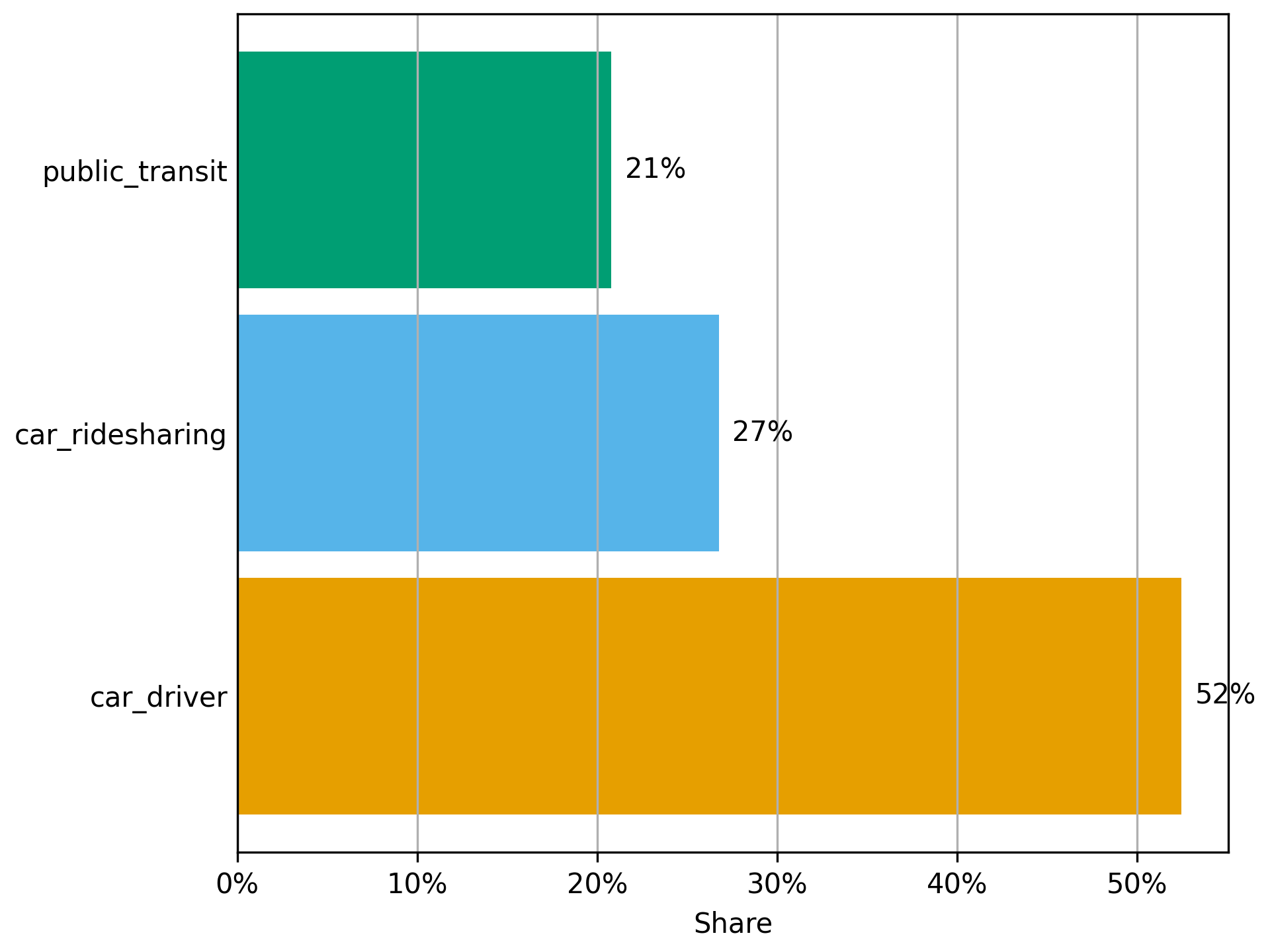
Figure 6. Mode shares with HOV lanes.
Matching constant
Coming soon.
Nested Logit for mode choice
Coming soon-ish.
Complete configuration with ridesharing
main_directory = "circular-city-ridesharing/"

random_seed = 123454321

[circular_network]
nb_radials = 8
nb_rings = 4
radius = 4000

[road_network]
[road_network.default_speed_limit]
"Radial 1" = 50
"Radial 2" = 50
"Radial 3" = 50
"Radial 4" = 50
"Ring 1" = 50
"Ring 2" = 70
"Ring 3" = 70
"Ring 4" = 70

[road_network.default_nb_lanes]
"Radial 1" = 1
"Radial 2" = 1
"Radial 3" = 1
"Radial 4" = 1
"Ring 1" = 2
"Ring 2" = 2
"Ring 3" = 2
"Ring 4" = 2

[road_network.capacities]
"Radial 1" = 1500
"Radial 2" = 2000
"Radial 3" = 2000
"Radial 4" = 2000
"Ring 1" = 2000
"Ring 2" = 2000
"Ring 3" = 2000
"Ring 4" = 2000

[road_network.hov_lanes]
"Ring 1" = 1
"Ring 2" = 1

[gravity_od_matrix]
exponential_decay = 0.07
trips_per_node = 8000

[mode_choice]
modes = ["car_driver", "car_ridesharing", "public_transit"]
model = "Logit"
mu = 1.0

[modes]
[modes.car_driver]
constant = 0.0
alpha = 10.0

[modes.car_ridesharing]
constant = 2.0
alpha = 11.0

[modes.public_transit]
constant = 2.0
alpha = 15.0
road_network_speed = 40

[departure_time_choice]
model = "ContinuousLogit"
mu = 1.0

[departure_time.linear_schedule]
beta = 6.0
gamma = 25.0
tstar = { mean = 08:00:00, std = 1800, distribution = "Uniform" }

[vehicle_types]
[vehicle_types.car]
ridesharing_passenger_count = 1.2

[fuel]
consumption_factor = 0.08
price = 1.8

[simulation]
period = [06:00:00, 10:00:00]
recording_interval = 300
learning_factor = 0.005
nb_iterations = 200

[metropolis_core]
exec_path = "execs/metropolis_cli"
References
de Palma, A., Kilani, M., & Lindsey, R. (2005). Congestion pricing on a road network: A study using the dynamic equilibrium simulator METROPOLIS. Transportation Research Part A: Policy and Practice, 39(7-9), 588-611.
Ghoslya, S., Javaudin, L., Palma, A. D., & Delle Site, P. (2025). Ride-sharing, congestion, departure-time and mode choices: A social optimum perspective. Available at SSRN 5465467.
Chambéry, France
Caution
This case study is incomplete and outdated.
Chambéry
Chambéry is a French city in the Savoie department, near the Alps. In 2021, the population of Chambéry was 59,856.
.JPG)
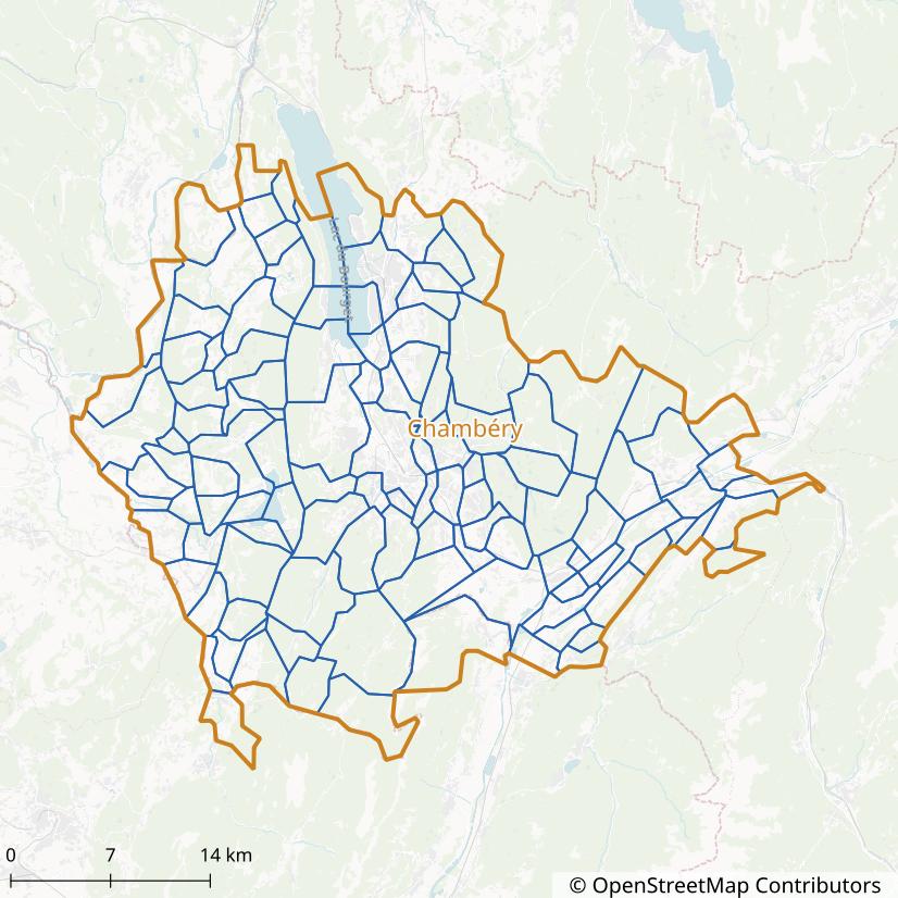
It is the largest city of the Chambéry Metropolitan area (Aire d’attraction de Chambéry) which has a population of 261,463 and an area of 1,147 km² (2021). The Metropolitan area of Chambéry consists of 115 French municipalities.
Chambéry has been selected for this case study due to its small size (reducing running times) and the availability of a recent travel survey (2022).
General Configuration
Before running the metropy pipeline, we need to create the TOML configuration file that specifies all the parameters of the simulation.
Create the config-chambery.toml file with the following content:
# File: config-chambery.toml
main_directory = "./chambery/output/"
crs = "EPSG:2154"
osm_file = "./chambery/data/rhone-alpes-250101.osm.pbf"
The main_directory variable represents the directory in which all the output files generated by
the pipeline will be saved.
The directory will be created automatically if it does not exist yet.
The crs variable represents the projected coordinate system to be used for all operations with
the spatial data (such as measuring the length of the road links).
The value "EPSG:2154" represents the Lambert-93 projection, which is
adapted for any area in Metropolitan France.
The osm_file variable specifies the path to the OpenStreetMap input file that will be used to
import the road and walking network.
We use the extract of the Rhône-Alpes French administrative region from 2025-01-01, that can be
downloaded from Geofabrik (click on
raw directory index to access older versions).
The Rhône-Alpes region is adapted for our case study given that the Chambéry urban area is full
contained within it.
Simulation Area
- Step:
simulation-area - Running time: 2 seconds
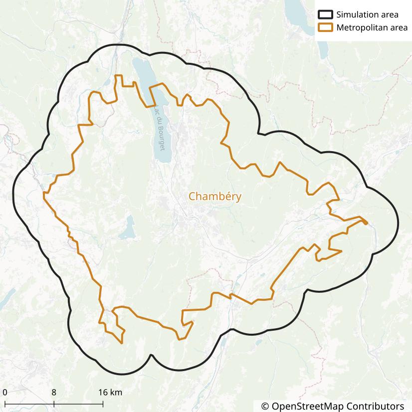
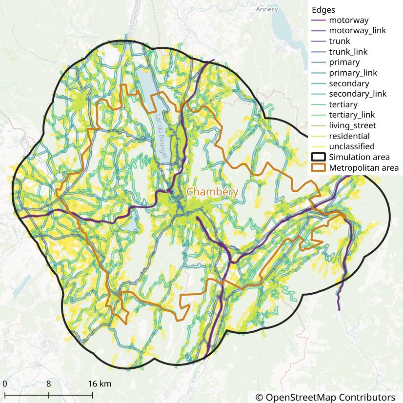
We define the simulation area as the Chambéry Metropolitan area (aire d’attraction) so that we get an area large enough to encompass most of the trips from and to Chambéry’s municipality.
To tell metropy to create the simulation area from the Chambéry Metropolitan area, add the following section to the configuration:
[simulation_area]
aav_name = "Chambéry"
buffer = 8000
The buffer = 8000 line tells metropy to extend the area by 8 kilometers in all directions.
This is used to include roads in the simulation that are not inside the Metropolitan area but that
could be taken when traveling between two municipalities within the area.
The output file ./chambery/output/simulation_area.parquet can be opened with QGIS to draw a map.
OpenStreetMap Road Import
- Step:
osm-road-import - Running time: 2 minutes
We use the osm-road-import step to import the road network from OpenStreetMap.
The step will read the osm_file variable previously defined.
Add the following section to the configuration:
[osm_road_import]
highways = [
"motorway",
"motorway_link",
"trunk",
"trunk_link",
"primary",
"primary_link",
"secondary",
"secondary_link",
"tertiary",
"tertiary_link",
"living_street",
"unclassified",
"residential",
]
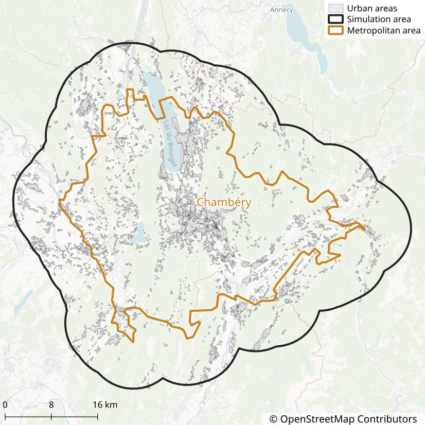
urban_landuse = [
"commercial",
"construction",
"education",
"industrial",
"residential",
"retail",
"village_green",
"recreation_ground",
"garages",
"religious",
]
urban_buffer = 50
The highways parameter lists all the OSM
highway tags to be imported.
In this case, all the standard tags are considered, including living streets, residential streets
and unclassified streets.
We do not consider however the service and road tags, which usually represent car park alleys or
other special roads we are not interested in.
The urban_landuse parameter lists all the OSM
landuse tags to be classified as urban.
The roads which are fully contained within urban areas will be classified as “urban”.
The urban areas are extended by 50 meters, through the urban_buffer parameter, so that roads
partially outside urban areas are also classified as “urban”.
After the step is completed, some statistics are reported in the file
./chambery/output/osm-road-import/output.txt.
They show that the imported road network has:
- 37 088 nodes
- 77 884 edges
- The total length of edges is 13 990 km
- 69.4 % of edges are classified as “urban”
- 2.2 % of edges are roundabouts
- 0.5 % of edges have traffic signals
- 1.0 % of edges have a stop sign
- 1.3 % of edges have a give-way sign
- 1.0 % of edges have tolls
- 68.7 % of edges do not have a speed limit reported
- 84.4 % of edges do not have a number of lanes reported
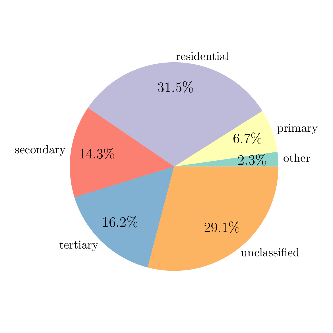
The directory ./chambery/output/graphs/osm-road-import/ also contains some graphs generated from
the imported data.
For example, the following pie chart reports the share of edges by road type (the category “other”
regroup all road types with few observations).
The two output files ./chambery/output/osm-road-import/edges_raw.parquet and
./chambery/output/osm-road-import/urban_areas.parquet can be opened with QGIS to draw a map of
edges…
and urban areas…
References
Steps
AdminExpressStep
Abstract Step to retrieve data from the ADMIN EXPRESS database.
Data is retrieved from local files when the
admin_express_directory parameter is defined,
otherwise data is requested from the WFS API.
AggregateResultsStep
Generates a JSON file with various aggregate results on the simulation.
NOTE: The developpement of this step is still in progress. More output will be added in the future. Do not hesitate to suggest additional output.
Currently available output:
- vehicle-kilometers (total, weighted by PCE, by mode)
- mode shares (by trip count, by trip Euclidean distance)
-
Parameters:
simulation_ratio -
Input files:
MetroVehicleTypesFile,TripResultsFile,TripsDistancesFile(optional) -
Output files:
AggregateOutputFile
AllFreeFlowTravelTimesStep
Computes travel time of the fastest path under (car) free-flow conditions, for all node pairs of the road network.
-
Input files:
RoadEdgesCleanFile,RoadEdgesFreeFlowTravelTimeFile -
Output files:
AllRoadFreeFlowTravelTimesFile
AllRoadDistancesStep
Computes distance of the shortest path, for all node pairs of the road network.
-
Input files:
RoadEdgesCleanFile -
Output files:
AllRoadDistancesFile
BicycleODNodesFromCoordinatesStep
Identifies nodes on the bicycle network to be used as origins and destinations of the trips.
First, this Step finds the nearest edge to the origin / destination coordinates.
Edges whose type is specified in the
forbidden_types parameter are excluded from
that search.
Then, the origin / destination node is either the source or target of that nearest edge,
whichever is closer.
-
Parameters:
bicycle_network.forbidden_types,crs -
Input files:
BicycleEdgesCleanFile,TripsDestinationsFile,TripsOriginsFile -
Output files:
TripsBicycleNodesFile
BicyclePreferencesFromPopulationStep
Generates the preference parameters of traveling by bicycle, for each trip, from constant values over population segments.
The following parameters are generated:
- constant: penalty of traveling by bicycle, per trip
- value of time / alpha: penalty per hour spent traveling by bicycle
The modes.bicycle.preferences_file parameter
must point to a Parquet or CSV file with the constant and/or alpha value for the population
segments.
The file can have the following columns:
constant: constant penalty for each bicycle trip (default is 0 when omitted)alphaorvalue_of_time: penalty per hour spent traveling by bicycle (default is 0 when omitted)mode: if present, only rows withmode = "bicycle"are used- any column representing persons’ characteristics from
PersonsFile
For example, to set different preferences for men and women, you can use the following CSV file:
mode,woman,constant,value_of_time
bicycle,true,-2,15
bicycle,false,-1,12
-
Parameters:
modes.bicycle.preferences_file -
Input files:
PersonsFile -
Output files:
BicyclePreferencesFile
BicyclePreferencesStep
Generates the preference parameters of traveling by bicycle, for each trip, from exogenous values.
The following parameters are generated:
- constant: penalty of traveling by bicycle, per trip
- value of time / alpha: penalty per hour spent traveling by bicycle
The values can be constant over trips or sampled from a specific distribution.
-
Parameters:
modes.bicycle.alpha,modes.bicycle.constant,random_seed -
Input files:
PersonsFile -
Output files:
BicyclePreferencesFile
BicycleTravelTimesFromDistanceStep
Computes travel time by bicycle for each trip, from a given distance and a constant speed.
The parameter modes.bicycle.distance.type specifies
how the bicycle distance is computed. For now, the only option is "pedestrian" which uses the
distance of the shortest path on the pedestrian network (Step
TripsPedestrianDistancesStep).
The parameter modes.bicycle.speed controls the speed at
which bicycles run.
If the parameter
modes.bicycle.distance.with_snap is set to
true, the snap distance at origin and destination is added to the bicycle travel time, with a
speed given by modes.bicycle.snap_speed (equal to
modes.bicycle.speed by default).
The snap distance corresponds to the distance between the trips’ origin and destination and the
network (See Step
PedestrianODNodesFromCoordinatesStep).
-
Parameters:
modes.bicycle.distance.type,modes.bicycle.distance.with_snap,modes.bicycle.snap_speed,modes.bicycle.speed -
Input files:
TripsPedestrianDistancesFile[ifmodes.bicycle.distance.typeis"pedestrian"],TripsPedestrianNodesFile[ifmodes.bicycle.distance.with_snapistrue] -
Output files:
BicycleTravelTimesFile
CarAccessEgressStep
Identifies the access and egress parts of car trips based on the primary road network.
For each car trip, this step determines:
- Access part: The sequence of edges taken before the first primary edge in the trip.
- Egress part: The sequence of edges taken after the last primary edge in the trip.
The access and egress parts are derived from the free-flow route of the trip and the set of primary edges. Trips that consist solely of primary edges or solely of secondary edges will not have access or egress parts.
The output includes the following information for each trip:
access_node: The node where the primary part of the trip begins.access_path: The list of edges in the access part.access_time: The total free-flow travel time for the access part.access_length: Length of the access part (meters).egress_node: The node where the primary part of the trip ends.egress_path: The list of edges in the egress part.egress_time: The total free-flow travel time for the egress part.egress_length: Length of the egress part (meters).
-
Input files:
RoadEdgesCleanFile,RoadEdgesFreeFlowTravelTimeFile,RoadEdgesPrimaryFlagFile,TripsCarFreeFlowTravelTimesFile -
Output files:
NonPrimaryCarTrips,PrimaryCarTripsAccessEgressFile
CarDriverPreferencesFromPopulationStep
Generates the preference parameters of traveling by car_driver, for each trip, from constant values over population segments.
The following parameters are generated:
- constant: penalty of traveling by car_driver, per trip
- value of time / alpha: penalty per hour spent traveling by car_driver
The modes.car_driver.preferences_file parameter
must point to a Parquet or CSV file with the constant and/or alpha value for the population
segments.
The file can have the following columns:
constant: constant penalty for each car_driver trip (default is 0 when omitted)alphaorvalue_of_time: penalty per hour spent traveling by car_driver (default is 0 when omitted)mode: if present, only rows withmode = "car_driver"are used- any column representing persons’ characteristics from
PersonsFile
For example, to set different preferences for men and women, you can use the following CSV file:
mode,woman,constant,value_of_time
car_driver,true,-2,15
car_driver,false,-1,12
-
Parameters:
modes.car_driver.preferences_file -
Input files:
PersonsFile -
Output files:
CarDriverPreferencesFile
CarDriverPreferencesStep
Generates the preference parameters of traveling by car_driver, for each trip, from exogenous values.
The following parameters are generated:
- constant: penalty of traveling by car_driver, per trip
- value of time / alpha: penalty per hour spent traveling by car_driver
The values can be constant over trips or sampled from a specific distribution.
-
Parameters:
modes.car_driver.alpha,modes.car_driver.constant,random_seed -
Input files:
PersonsFile -
Output files:
CarDriverPreferencesFile
CarDriverWithPassengersPreferencesFromPopulationStep
Generates the preference parameters of traveling by car_driver_with_passengers, for each trip, from constant values over population segments.
The following parameters are generated:
- constant: penalty of traveling by car_driver_with_passengers, per trip
- value of time / alpha: penalty per hour spent traveling by car_driver_with_passengers
The modes.car_driver_with_passengers.preferences_file parameter
must point to a Parquet or CSV file with the constant and/or alpha value for the population
segments.
The file can have the following columns:
constant: constant penalty for each car_driver_with_passengers trip (default is 0 when omitted)alphaorvalue_of_time: penalty per hour spent traveling by car_driver_with_passengers (default is 0 when omitted)mode: if present, only rows withmode = "car_driver_with_passengers"are used- any column representing persons’ characteristics from
PersonsFile
For example, to set different preferences for men and women, you can use the following CSV file:
mode,woman,constant,value_of_time
car_driver_with_passengers,true,-2,15
car_driver_with_passengers,false,-1,12
-
Parameters:
modes.car_driver_with_passengers.preferences_file -
Input files:
PersonsFile -
Output files:
CarDriverWithPassengersPreferencesFile
CarDriverWithPassengersPreferencesStep
Generates the preference parameters of traveling by car_driver_with_passengers, for each trip, from exogenous values.
The following parameters are generated:
- constant: penalty of traveling by car_driver_with_passengers, per trip
- value of time / alpha: penalty per hour spent traveling by car_driver_with_passengers
The values can be constant over trips or sampled from a specific distribution.
-
Parameters:
modes.car_driver_with_passengers.alpha,modes.car_driver_with_passengers.constant,random_seed -
Input files:
PersonsFile -
Output files:
CarDriverWithPassengersPreferencesFile
CarFuelStep
Generates the fuel consumption and price of each car trips by applying a constant emission factor to the free-flow fastest-path length, combined with a fuel price.
-
Parameters:
fuel.consumption_factor,fuel.price -
Input files:
TripsCarFreeFlowTravelTimesFile -
Output files:
CarFuelFile
CarPassengerPreferencesFromPopulationStep
Generates the preference parameters of traveling by car_passenger, for each trip, from constant values over population segments.
The following parameters are generated:
- constant: penalty of traveling by car_passenger, per trip
- value of time / alpha: penalty per hour spent traveling by car_passenger
The modes.car_passenger.preferences_file parameter
must point to a Parquet or CSV file with the constant and/or alpha value for the population
segments.
The file can have the following columns:
constant: constant penalty for each car_passenger trip (default is 0 when omitted)alphaorvalue_of_time: penalty per hour spent traveling by car_passenger (default is 0 when omitted)mode: if present, only rows withmode = "car_passenger"are used- any column representing persons’ characteristics from
PersonsFile
For example, to set different preferences for men and women, you can use the following CSV file:
mode,woman,constant,value_of_time
car_passenger,true,-2,15
car_passenger,false,-1,12
-
Parameters:
modes.car_passenger.preferences_file -
Input files:
PersonsFile -
Output files:
CarPassengerPreferencesFile
CarPassengerPreferencesStep
Generates the preference parameters of traveling by car_passenger, for each trip, from exogenous values.
The following parameters are generated:
- constant: penalty of traveling by car_passenger, per trip
- value of time / alpha: penalty per hour spent traveling by car_passenger
The values can be constant over trips or sampled from a specific distribution.
-
Parameters:
modes.car_passenger.alpha,modes.car_passenger.constant,random_seed -
Input files:
PersonsFile -
Output files:
CarPassengerPreferencesFile
CarRidesharingPreferencesFromPopulationStep
Generates the preference parameters of traveling by car_ridesharing, for each trip, from constant values over population segments.
The following parameters are generated:
- constant: penalty of traveling by car_ridesharing, per trip
- value of time / alpha: penalty per hour spent traveling by car_ridesharing
The modes.car_ridesharing.preferences_file parameter
must point to a Parquet or CSV file with the constant and/or alpha value for the population
segments.
The file can have the following columns:
constant: constant penalty for each car_ridesharing trip (default is 0 when omitted)alphaorvalue_of_time: penalty per hour spent traveling by car_ridesharing (default is 0 when omitted)mode: if present, only rows withmode = "car_ridesharing"are used- any column representing persons’ characteristics from
PersonsFile
For example, to set different preferences for men and women, you can use the following CSV file:
mode,woman,constant,value_of_time
car_ridesharing,true,-2,15
car_ridesharing,false,-1,12
-
Parameters:
modes.car_ridesharing.preferences_file -
Input files:
PersonsFile -
Output files:
CarRidesharingPreferencesFile
CarRidesharingPreferencesStep
Generates the preference parameters of traveling by car_ridesharing, for each trip, from exogenous values.
The following parameters are generated:
- constant: penalty of traveling by car_ridesharing, per trip
- value of time / alpha: penalty per hour spent traveling by car_ridesharing
The values can be constant over trips or sampled from a specific distribution.
-
Parameters:
modes.car_ridesharing.alpha,modes.car_ridesharing.constant,random_seed -
Input files:
PersonsFile -
Output files:
CarRidesharingPreferencesFile
CircularNetworkStep
Generates a toy road network of circular form with radial and ring roads.
The network is inspired by de Palma, A., Kilani, M., & Lindsey, R. (2005). Congestion pricing on a road network: A study using the dynamic equilibrium simulator METROPOLIS. Transportation Research Part A: Policy and Practice, 39(7-9), 588-611.
The network has a center node, called “CBD”.
From the center, bidirectional radial roads are going in all directions.
The number of radial roads is controled by the nb_radials parameters and they are evenly
spaced (in the polar dimension).
At fixed distances from the center (controled by the parameter radius), bidirectional rings
are connecting the radial roads together.
The number of rings is controled by the nb_rings parameter.
There is one node at each crossing of a ring road with a radial road.
The number of nodes is thus nb_radials * nb_rings + 1.
The number of edges is 4 * nb_radials * nb_rings.
Node ids are set to "{D}-{i}", where D is the direction (N, S, E, W, NW, NE, SW, SE, or D1,
D2, etc. when the number of radials is different from 2, 4, or 8) and i is the ring index
(starting at 1).
For example, node "NW-1" is at the intersection of the Northwest radial with the first ring
(closest ring to the center).
Node "D1-2" is at the intersection of the first radial road (radial roads are generated
starting from the east direction and going in a counterclockwise direction, like the unit
circle) with the second ring.
By convention, the center node is denoted "CBD".
Edge ids for radial roads are set to "In{i}-{D}" for edges going toward the center and
"Out{i}-{D}" for edges going away from the center, with the same definition of D and i
than for the nodes.
For example, edge "In2-S" is the radial edge on the South axis, between the first and second
ring (its source node is "S-2" and its target node is "S-1").
Edge ids for ring roads are set to {D1}-{D2}-{i}, where D1 is the direction the edge is
starting from, D2 is the direction the edge is going to, and i is the ring index.
For example, edge "S-SE-1" is the ring edge from node "S-1" to node "SE-1".
Road types are set to "Radial {i}" for radial roads and "Ring {i}" for ring roads.
The parameter with_ramps allows to split each node of the road network (except the CBD node)
in four different nodes (inner, outer, left, and right) connected by edges representing entry /
exit ramps in and out of highways.
-
Parameters:
circular_network.entry_ramps_length,circular_network.exit_ramps_length,circular_network.nb_radials,circular_network.nb_rings,circular_network.radial_inter_ramp_length,circular_network.radius,circular_network.resolution,circular_network.ring_inter_ramp_length,circular_network.with_ramps -
Output files:
RoadEdgesRawFile
ConvergencePlotStep
Generates various graphs to analyze the convergence of the simulation.
-
Input files:
IterationResultsFile -
Output files:
ExpectedRoadTravelTimesConvergencePlotFile,MeanSurplusConvergencePlotFile,RouteLengthDiffConvergencePlotFile,SimulatedRoadTravelTimesConvergencePlotFile,TourDepartureTimeConvergencePlotFile
CustomODMatrixStep
Generates car driver origin-destination pairs from the provided origin-destination matrix.
The origin-destination matrix is provided in a CSV or Parquet file with the following columns:
origin: id of the origin node,destination: id of the destination node,size: number of trips to be generated from origin to destination.
The size variable can be integers or floats.
For float values, stochastic rounding is used to convert the value to an integer: e.g., 3.3 is
converted to 3 with probability 70% and to 4 with probability 30%.
-
Parameters:
od_matrix.file,random_seed -
Input files:
RoadEdgesCleanFile -
Output files:
TripsRoadNodesFile
CustomRoadImportStep
Imports a road network from a geospatial file.
The file must have the same schema has the RawEdgesFile.
-
Parameters:
custom_road_import.edges_file -
Output files:
RoadEdgesRawFile
CustomZonesStep
Reads zones from a geospatial file.
The input file can have these three columns:
geometry: Polygon or MultiPolygon of the zoneszone_id: Identifier of the zone (integer or sting)name: Name of the zone (string)
The two first columns are mandatory.
-
Parameters:
zones.custom_zones -
Output files:
ZonesFile
EdgesFreeFlowTravelTimesStep
Generates free-flow travel times for each edge of the road network.
The free-flow travel time of an edge is:
constant_penalty + length / speed
-
Input files:
RoadEdgesCleanFile,RoadEdgesPenaltiesFile(optional) -
Output files:
RoadEdgesFreeFlowTravelTimeFile
EqasimImportStep
Imports a synthetic population from the output of the Eqasim pipeline.
To use this step, you first need to generate a synthetic population following the instructions here: https://github.com/eqasim-org/eqasim-france.
A few extra steps need to be done for Pymetropolis:
- Set the
departementsorregionsconfiguration parameter so that it englobs the simulation area. Pymetropolis will automatically restricts the population to the simulation area (if defined). - Use parquet and geoparquet as output formats (optional):
output_formats: - "parquet" - "geoparquet" - Use MobiSurvStd for the Household Travel Survey (optional):
hts: mobisurvstd mobisurvstd: path: path/to/compatible/hts/ - Use
urban_typeandprofessional_activityas extra matching attributes (optional):use_urban_type: true matching_attributes: ["professional_activity", "urban_type", "*default*"]- Add extra attributes to the generated persons (optional):
extra_enriched_attributes:
  - "education_level"
  - "detailed_education_level"
- Add extra attributes to the generated persons (optional):
- Do not activate mode choice (unused):
mode_choice: false
-
Parameters:
crs,random_seed,synthetic_population.eqasim_output,synthetic_population.fraction -
Input files:
SimulationAreaFile(optional) -
Output files:
HouseholdsFile,HouseholdsHomesFile,PersonsFile,TripsDestinationsFile,TripsFile,TripsOriginsFile
ExogenousBicycleEdgeCostsStep
Generates costs for the bicycle network edges, from exogenous values.
-
Input files:
BicycleEdgesCleanFile -
Output files:
BicycleEdgesCostsFile
ExogenousCapacitiesStep
Generates bottleneck capacities for the road network edges, from exogenous values.
The bottleneck capacities can be:
- constant over edges
- constant by edge type
- constant by combinations of edge type and urban flag
-
Parameters:
road_network.capacities -
Input files:
RoadEdgesCleanFile,RoadEdgesUrbanFlagFile[if default capacities rely on the urban flag] -
Output files:
RoadEdgesCapacitiesFile
ExogenousEdgePenaltiesStep
Generates travel time penalties for the road network edges, from exogenous values.
The penalties can be:
- constant over edges
- constant by edge type
- constant by combinations of edge type and urban flag
-
Parameters:
road_network.penalties -
Input files:
RoadEdgesCleanFile,RoadEdgesUrbanFlagFile[if default penalties rely on the urban flag] -
Output files:
RoadEdgesPenaltiesFile
FrenchHouseholdsHomesZonesStep
Identifies the geographic zones where households’ homes are located in the French zoning system.
The French zoning system uses multiple levels of geographic zones:
- Zone 1: Region
- Zone 2: Department
- Zone 3: EPCI (Établissement Public de Coopération Intercommunale)
- Zone 4: INSEE commune
- Zone 5: IRIS
Check the AdminExpressStep and IRISStep
abstract steps to know how to configure this step.
-
Parameters:
ign.admin_express_directory,ign.api_communes_service_name,ign.api_iris_service_name,ign.api_wfs_url,ign.contours_iris_directory -
Input files:
HouseholdsHomesFile -
Output files:
HouseholdsZonesFile
FrenchTripsZonesStep
Identifies the geographic zones where trips’ origins and destinations are located in the French zoning system.
The French zoning system uses multiple levels of geographic zones:
- Zone 1: Region
- Zone 2: Department
- Zone 3: EPCI (Établissement Public de Coopération Intercommunale)
- Zone 4: INSEE commune
- Zone 5: IRIS
Check the AdminExpressStep and IRISStep
abstract steps to know how to configure this step.
-
Parameters:
ign.admin_express_directory,ign.api_communes_service_name,ign.api_iris_service_name,ign.api_wfs_url,ign.contours_iris_directory -
Input files:
TripsDestinationsFile,TripsOriginsFile -
Output files:
TripsZonesFile
GenericPopulationStep
Generates a population (persons and trips) from a list of car-driver origin-destination pairs.
Each person has a single trip.
-
Input files:
TripsRoadNodesFile -
Output files:
PersonsFile,TripsFile
GravityODMatrixStep
Generates car driver origin-destination pairs by generating trips from a gravity model.
The model is based on de Palma, A., Kilani, M., & Lindsey, R. (2005). Congestion pricing on a road network: A study using the dynamic equilibrium simulator METROPOLIS. Transportation Research Part A: Policy and Practice, 39(7-9), 588-611.
The total number of trips generated from each node is fixed (parameter trips_per_node).
Then, the number of trips generated from node \(i\) to node \(j\) is proportional to:
\[ e^{-\lambda \cdot {tt}^0} \]
where \(\lambda\) is the decay rate (parameter exponential_decay) and \({tt}^0\) is the
free-flow travel time by car from node \(i\) to node \(j\).
-
Parameters:
gravity_od_matrix.exponential_decay,gravity_od_matrix.nodes_regex,gravity_od_matrix.trips_per_node,random_seed -
Input files:
AllRoadFreeFlowTravelTimesFile -
Output files:
TripsRoadNodesFile
GridNetworkStep
Generates a toy road network from a grid.
The network is defined by a number of rows and columns.
The first node is located at the bottom left, at coordinates (0, 0).
Then, the node on the i-th column and j-th row has coordinates (i - 1, j - 1).
The total number of nodes is nb_columns * nb_rows.
By default, edges are bidirectional, connecting all adjacent nodes.
The total number of edges is thus
2 * nb_columns * (nb_rows - 1) + 2 * nb_rows * (nb_columns - 1).
The length parameter control the length of all edges.
With the parameters left_to_right, right_to_left, bottom_to_top, and top_to_bottom (by
default all equal to true), it is possible to disable the creation of edges in some direction.
For example, if right_to_left is set to false, all horizontal edges will be unidirectional
(towards increasing x coordinate).
Be careful, if the edges are not all bidirectional, the grid network is not strongly connected which can cause issue later on in the simulation.
A network of successive roads can be created by setting nb_rows to 1, nb_columns to the
desired number of roads + 1, and right_to_left to false.
Node ids are set to "Node_{x}_{y}", where x is the index of the column and y is the index
of the row (starting at 0).
For row edges, ids are set to "Row_{y}:{x1}to{x2}" for row y, when connecting column x1 to
column x2.
For column edges, ids are set to "Col_{x}:{y1}to{y2}" for column x, when connecting row x1
to row x2.
Road types are set to the edge direction: "LeftToRight", "RightToLeft", "TopToBottom", or
"BottomToTop".
-
Parameters:
grid_network.bottom_to_top,grid_network.left_to_right,grid_network.length,grid_network.nb_columns,grid_network.nb_rows,grid_network.right_to_left,grid_network.top_to_bottom -
Output files:
RoadEdgesRawFile
HomogeneousTstarStep
Generates the desired start time of the activity following each trip, from exogenous values.
The desired start times can be constant over trips or sampled from a specific distribution. It is recommended to only use this Step when each person has one trip only.
This Step should be combined with a Step that generate schedule-utility parameters.
-
Parameters:
departure_time.linear_schedule.tstar,random_seed -
Input files:
TripsFile -
Output files:
TstarsFile
IRISStep
Abstract Step to retrieve data from the Contours IRIS database.
Data is retrieved from local file when the
contours_iris_directory parameter is defined,
otherwise data is requested from the WFS API.
IterationResultsStep
Reads the iteration-level results from the Metropolis-Core simulation and produces a clean file for the results.
-
Input files:
MetroIterationResultsFile -
Output files:
IterationResultsFile
LinearScheduleFromPurposeStep
Generates the preference parameters for schedule-delay utility of each trip, from constant values over purposes.
The following parameters are generated:
- beta: the penalty for starting the following activity earlier than the desired time
- gamma: the penalty for starting the following activity earlier than the desired time
- delta: the length of the desired time window
The
departure_time.linear_schedule.preferences_file
parameter must point to a Parquet or CSV file with the beta, gamma and/or delta values for each
purpose.
The file can have the following columns:
purpose: purpose for which the given values applybeta: early penalty, in euros per hour (default is 0 when omitted)gamma: late penalty, in euros per hour (default is 0 when omitted)delta: desired-time window length, given in number of seconds or directly as Duration dtype (default is 0 when omitted)
For example, to set the beta and gamma values for work and education purposes:
purpose,beta,gamma
work,5,15
education,4,10
-
Parameters:
departure_time.linear_schedule.preferences_file -
Input files:
TripsFile -
Output files:
LinearScheduleFile
LinearScheduleStep
Generates the preference parameters for schedule-delay utility of each trip, using a linear-penalty model (à la Arnott, de Palma, Lindsey), from exogenous values.
For each trip, the following parameters are created:
- beta: the penalty for starting the following activity earlier than the desired time
- gamma: the penalty for starting the following activity earlier than the desired time
- delta: the length of the desired time window
The values can be constant over trips or sampled from a specific distribution.
This Step should be combined with a Step that generate desired activity start times.
-
Parameters:
departure_time.linear_schedule.beta,departure_time.linear_schedule.delta,departure_time.linear_schedule.gamma,random_seed -
Input files:
TripsFile -
Output files:
LinearScheduleFile
ODMatrixEachStep
Generates car driver origin-destination pairs by generating a fixed number of trips for each node pair of the road network.
Nodes selected as eligible origins are all nodes with at least one outgoing edge. Nodes selected as eligible destinations are all nodes with at least one incoming edge.
If the road network is not strongly connected, there is no guarantee that all the origin-destination pairs generated are feasible (i.e., there is a path from origin to destination).
-
Parameters:
node_od_matrix.each,random_seed -
Input files:
RoadEdgesCleanFile -
Output files:
TripsRoadNodesFile
OpenStreetMapBicycleImportStep
Imports a bicycle network from OpenStreetMap data.
Edges of the bicycle network are read from the OpenStreetMap ways with tag highway:*.
The osm_bicycle_import.highways parameter is used
to define the highway values which are part of the bicycle network. For example, values
"cycleway" and "path" should usually be included, while value "motorway" should be
excluded as it does not represent ways accessible by bicycles.
In addition to the highways parameter, this step requires both the
osm_file and crs parameters to be set.
For example, to import the cycleways in Paris, you can use:
osm_file = "path/to/paris.osm.pbf"
crs = "epsg:2154"

[osm_bicycle_import]
highways = [
  "tertiary",
  "tertiary_link",
  "residential",
  "cycleway",
  "path",
]
An OpenStreetMap way is selected as valid cycleway edge if it satisfies all the conditions below:
- Tag
highwaymatches one of the value given inhighwaysparameter. - The way has no tag
bicycleor tagbicycleis not"no". - The way’s geometry is a valid LineString.
- The way intersects with the simulation area (if
simulation_area_filteristrue).
When filtering with the simulation area, the
simulation_area_buffer parameter can
be used to extend or shrink the area by a given distance.
This can be useful to include edges outside the area that might be used when traveling between
two points inside the area.
Various processing operations are done to clean the edges:
- Duplicate
oneway=falseways in two opposing edges. - Split ways at nodes where another way is intersecting.
Edges attributes are defined as follows: TODO
edge_id: OSM id of the way, with “r” appended if the edge is going backward, with “-[idx]” appended if the edge is split in multiple segments (withidxthe segment index).source: OSM id of the source node.target: OSM id of the target node.original_id: OSM id of the way (note that values are generally not unique).length: computed as geometric operation on the ways’ LineString, after conversion to the simulation CRS.edge_type:highwaytag value.name:nametag value if any, otherwiseaddr:streettag value if any, otherwisereftag value if any.speed_limit: read frommaxspeed,maxspeed:forward, ormaxspeed:backwardtag, as appropriate.lanes: read fromlanes,lanes:forward, orlanes:backwardtag, as appropriate.oneway:onewaytag value.roundabout:Trueifjunction=roundabout.toll:Trueiftoll=yes.give_way: way has a node withhighway=give_way, in the correct direction.stop: way has a node withhighway=stop, in the correct direction.traffic_signals: way has a node withhighway=traffic_signals, in the correct direction.
-
Parameters:
crs,osm_bicycle_import.highways,osm_bicycle_import.simulation_area_buffer,osm_bicycle_import.simulation_area_filter,osm_file -
Input files:
SimulationAreaFile[ifsimulation_area_filteris set totrue] -
Output files:
BicycleEdgesRawFile
OpenStreetMapPedestrianImportStep
Imports a pedestrian network from OpenStreetMap data.
Edges of the pedestrian network are read from the OpenStreetMap ways with tag highway:*.
The osm_pedestrian_import.highways parameter is
used to define the highway values which are part of the pedestrian network. For example,
values "footway" and "path" should usually be included, while value "motorway" should be
excluded as motorways are generally not allowed for pedestrians.
In addition to the highways parameter, this step requires both the
osm_file and crs parameters to be set.
For example, to import the pedestrian network of Paris, you can use:
osm_file = "path/to/paris.osm.pbf"
crs = "epsg:2154"

[osm_pedesrian_import]
highways = [
    "primary",
    "primary_link",
    "secondary",
    "secondary_link",
    "tertiary",
    "tertiary_link",
    "living_street",
    "unclassified",
    "residential",
    "road",
    "service",
    "track",
    "footway",
    "path",
    "pedestrian",
]
An OpenStreetMap way is selected as valid pedestrian-network edge if it satisfies all the conditions below:
- Tag
highwaymatches one of the value given inhighwaysparameter. - The way has no tag
accessor tagaccessis not"private". - The way’s geometry is a valid LineString.
- The way intersects with the simulation area (if
simulation_area_filteristrue).
When filtering with the simulation area, the
simulation_area_buffer parameter
can be used to extend or shrink the area by a given distance.
This can be useful to include edges outside the area that might be used when traveling between
two points inside the area.
Edges attributes are defined as follows:
edge_id: OSM id of the way, with “r” appended if the edge is going backward, with “-[idx]” appended if the edge is split in multiple segments (withidxthe segment index).source: OSM id of the source node.target: OSM id of the target node.original_id: OSM id of the way (note that values are generally not unique).length: computed as geometric operation on the ways’ LineString, after conversion to the simulation CRS.edge_type:highwaytag value.name:nametag value if any, otherwiseaddr:streettag value if any, otherwisereftag value if any.
-
Parameters:
crs,osm_file,osm_pedestrian_import.highways,osm_pedestrian_import.simulation_area_buffer,osm_pedestrian_import.simulation_area_filter -
Input files:
SimulationAreaFile[ifsimulation_area_filteris set totrue] -
Output files:
PedestrianEdgesRawFile
OpenStreetMapRoadImportStep
Imports a road network from OpenStreetMap data.
Edges of the road network are read from the OpenStreetMap ways with tag highway:*.
The osm_road_import.highways parameter is used to
define the highway values which are part of the road network. For example, values "motorway"
and "motorway_link" should usually be included, while value "footway" should be excluded as
it does not represent ways accessible by road vehicles.
In addition to the highways parameter, this step requires both the
osm_file and crs parameters to be set.
For example, to import the major roads of Paris, you can use:
osm_file = "path/to/paris.osm.pbf"
crs = "epsg:2154"

[osm_road_import]
highways = [
  "motorway",
  "motorway_link",
  "trunk",
  "trunk_link",
  "primary",
  "primary_link",
  "secondary",
  "secondary_link",
]
An OpenStreetMap way is selected as valid road-network edge if it satisfies all the conditions below:
- Tag
highwaymatches one of the value given inhighwaysparameter. - The way has no tag
accessor tagaccessmatches one of the value given inallowed_access. - The way’s geometry is a valid LineString.
- The way intersects with the simulation area (if
simulation_area_filteristrue).
By default, the allowed tags for access are yes, permissive (non-public roads with allowed
access), and destination (allowed for local traffic only).
When filtering with the simulation area, the
simulation_area_buffer parameter can be
used to extend or shrink the area by a given distance.
This can be useful to include edges outside the area that might be used when traveling between
two points inside the area.
Various processing operations are done to clean the edges:
- Duplicate
oneway=falseways in two opposing edges. - Split ways at nodes where another way is intersecting.
Edges attributes are defined as follows:
edge_id: OSM id of the way, with “r” appended if the edge is going backward, with “-[idx]” appended if the edge is split in multiple segments (withidxthe segment index).source: OSM id of the source node.target: OSM id of the target node.original_id: OSM id of the way (note that values are generally not unique).length: computed as geometric operation on the ways’ LineString, after conversion to the simulation CRS.edge_type:highwaytag value.name:nametag value if any, otherwiseaddr:streettag value if any, otherwisereftag value if any.speed_limit: read frommaxspeed,maxspeed:forward, ormaxspeed:backwardtag, as appropriate.lanes: read fromlanes,lanes:forward, orlanes:backwardtag, as appropriate.oneway:onewaytag value.roundabout:Trueifjunction=roundabout.toll:Trueiftoll=yes.give_way: way has a node withhighway=give_way, in the correct direction.stop: way has a node withhighway=stop, in the correct direction.traffic_signals: way has a node withhighway=traffic_signals, in the correct direction.
-
Parameters:
crs,osm_file,osm_road_import.allowed_access,osm_road_import.highways,osm_road_import.simulation_area_buffer,osm_road_import.simulation_area_filter -
Input files:
SimulationAreaFile[ifsimulation_area_filteris set totrue] -
Output files:
RoadEdgesRawFile
OpenStreetMapUrbanAreasStep
Identifies urban areas from OpenStreetMap data.
Urban areas are read from the OpenStreetMap areas with tag landuse:*.
The osm_urban_areas.urban_landuse_tags
parameter is used to define the landuse values which are considered as urban.
For example, values "residential", "industrial", "commercial", or "retail" should
generally be included.
In addition to the urban_landuse_tags parameter, this step requires both the
osm_file and crs parameters to be set.
For example, to identifies the urban areas of Brittany, you can use:
osm_file = "path/to/brittany.osm.pbf"
crs = "epsg:2154"

[osm_urban_areas]
urban_landuse_tags = [
  "residential",
  "industrial",
  "commercial",
  "retail",
]
The osm_urban_areas.buffer parameter can be used to
extend (positive values) or shrink (negative values) the areas.
-
Parameters:
crs,osm_file,osm_urban_areas.buffer,osm_urban_areas.urban_landuse_tags -
Input files:
SimulationAreaFile(optional) -
Output files:
UrbanAreasFile
OutsideOptionPreferencesStep
Generates the preference parameters of the outside option alternative from exogenous values.
The following parameters are generated:
- constant: utility of choosing the outside option alternative
- value of time / alpha: penalty per hour spent traveling for the outside option (this usually irrelevant as the outside option does not imply traveling)
The values can be constant over tours or sampled from a specific distribution.
-
Parameters:
modes.outside_option.alpha,modes.outside_option.constant,random_seed -
Input files:
OutsideOptionTravelTimesFile(optional),TripsFile -
Output files:
OutsideOptionPreferencesFile
OutsideOptionTravelTimesFromRoadDistancesStep
Generates travel times for the outside option alternatives by applying a constant speed to the shortest-path distances of the car-driver trips.
If a tour has multiple trips, the outside option travel time of the tour depends on the sum of the shortest-path distances of all trips.
-
Parameters:
modes.outside_option.road_network_speed -
Input files:
TripsCarFreeFlowTravelTimesFile,TripsFile -
Output files:
OutsideOptionTravelTimesFile
PedestrianODNodesFromCoordinatesStep
Identifies nodes on the pedestrian network to be used as origins and destinations of the trips.
First, this Step finds the nearest edge to the origin / destination coordinates.
Edges whose type is specified in the
forbidden_types parameter are excluded from
that search.
Then, the origin / destination node is either the source or target of that nearest edge,
whichever is closer.
-
Parameters:
crs,pedestrian_network.forbidden_types -
Input files:
PedestrianEdgesCleanFile,TripsDestinationsFile,TripsOriginsFile -
Output files:
TripsPedestrianNodesFile
PopulationFromTripCoordinatesStep
Generates a population (persons and trips) from a list of trips with origin / destination coordinates.
Each person has a single trip.
The input file must have columns: trip_id, origin_lng, origin_lat, destination_lng,
destination_lat.
-
Parameters:
crs,population.trip_coordinates_file -
Output files:
PersonsFile,TripsDestinationsFile,TripsFile,TripsOriginsFile
PostprocessBicycleNetworkStep
Performs some operations on the “raw” bicycle network to make it suitable for simulation.
The operations performed are:
- Remove all parallel edges (edges with same source and target nodes), keeping only the edge
of minimum distance. This is only done if
remove_duplicatesistrue. - Keep only the largest strongly connected component of the bicycle-network graph. This
ensures that all origin-destination pairs are feasible. This is only done if
ensure_connectedistrue. - Set edge ids to
1,...,n, wherenis the number of edges. This is only done ifreindexistrue.
-
Parameters:
bicycle_network.ensure_connected,bicycle_network.reindex,bicycle_network.remove_duplicates -
Input files:
BicycleEdgesRawFile -
Output files:
BicycleEdgesCleanFile
PostprocessPedestrianNetworkStep
Performs some operations on the “raw” pedestrian network to make it suitable for simulation.
The operations performed are:
- Remove all parallel edges (edges with same source and target nodes), keeping only the edge
of minimum distance. This is only done if
remove_duplicatesistrue. - Keep only the largest strongly connected component of the pedestrian-network graph. This
ensures that all origin-destination pairs are feasible. This is only done if
ensure_connectedistrue. - Set edge ids to
1,...,n, wherenis the number of edges. This is only done ifreindexistrue.
-
Parameters:
pedestrian_network.ensure_connected,pedestrian_network.reindex,pedestrian_network.remove_duplicates -
Input files:
PedestrianEdgesRawFile -
Output files:
PedestrianEdgesCleanFile
PostprocessRoadNetworkStep
Performs some operations on the “raw” road network to make it suitable for simulation.
The operations performed are:
- Replace NULL values with defaults for columns
speed_limit,lanes,hov_lanes, and all the boolean columns. - Remove all parallel edges (edges with same source and target nodes), keeping only the edge
of minimum free-flow travel time. This is only done if
remove_duplicatesistrue. - Keep only the largest strongly connected component of the road-network graph. This ensures
that all origin-destination pairs are feasible. This is only done if
ensure_connectedistrue. - Set edge ids to
1,...,n, wherenis the number of edges. This is only done ifreindexistrue. - Set a minimum value for the number of lanes, speed limit, and length of edges.
- Compute in- and out-degrees of nodes.
The default values for speed_limit and lanes can be specified as
- constant value over edges
- constant value by edge type
- constant value by combinations of edge type and urban flag
-
Parameters:
road_network.default_lanes,road_network.default_speed_limit,road_network.ensure_connected,road_network.hov_lanes,road_network.min_lanes,road_network.min_length,road_network.min_speed_limit,road_network.reindex,road_network.remove_duplicates -
Input files:
RoadEdgesRawFile,RoadEdgesUrbanFlagFile[if default values rely on the urban flag] -
Output files:
RoadEdgesCleanFile
PublicTransitPreferencesFromPopulationStep
Generates the preference parameters of traveling by public_transit, for each trip, from constant values over population segments.
The following parameters are generated:
- constant: penalty of traveling by public_transit, per trip
- value of time / alpha: penalty per hour spent traveling by public_transit
The modes.public_transit.preferences_file parameter
must point to a Parquet or CSV file with the constant and/or alpha value for the population
segments.
The file can have the following columns:
constant: constant penalty for each public_transit trip (default is 0 when omitted)alphaorvalue_of_time: penalty per hour spent traveling by public_transit (default is 0 when omitted)mode: if present, only rows withmode = "public_transit"are used- any column representing persons’ characteristics from
PersonsFile
For example, to set different preferences for men and women, you can use the following CSV file:
mode,woman,constant,value_of_time
public_transit,true,-2,15
public_transit,false,-1,12
-
Parameters:
modes.public_transit.preferences_file -
Input files:
PersonsFile -
Output files:
PublicTransitPreferencesFile
PublicTransitPreferencesStep
Generates the preference parameters of traveling by public_transit, for each trip, from exogenous values.
The following parameters are generated:
- constant: penalty of traveling by public_transit, per trip
- value of time / alpha: penalty per hour spent traveling by public_transit
The values can be constant over trips or sampled from a specific distribution.
-
Parameters:
modes.public_transit.alpha,modes.public_transit.constant,random_seed -
Input files:
PersonsFile -
Output files:
PublicTransitPreferencesFile
PublicTransitTravelTimesFromRoadDistancesStep
Generates travel times for the public-transit trips by applying a constant speed to the shortest-path distances of the car-driver trips.
-
Parameters:
modes.public_transit.road_network_speed -
Input files:
TripsCarFreeFlowTravelTimesFile -
Output files:
TripsPublicTransitItinerariesFile
RoadEdgesVariablesStep
This Step generates edge-level variables to be used in the calibration process.
-
Parameters:
road_network.calibration_variables -
Input files:
RoadEdgesCleanFile,RoadEdgesUrbanFlagFile(optional) -
Output files:
RoadEdgesVariablesFile
RoadNetworkCongestionFunctionPlotsStep
Generates plots of expected and simulated congestion function global over the entire road network.
-
Input files:
MetroExpectedTravelTimeFunctionsFile,MetroSimulatedTravelTimeFunctionsFile,RoadEdgesFreeFlowTravelTimeFile -
Output files:
ExpectedRoadNetworkCongestionFunctionPlotFile,SimulationRoadNetworkCongestionFunctionPlotFile
RoadNetworkPrimaryEdgesStep
Identifies the edges which are part of the “primary” road network.
Only primary edges are simulated in Metropolis-Core, whereas the secondary edges are supposed to always be under free-flow conditions. By default, all edges are considered “primary”.
You can use the secondary_types parameter to
define the list of edges’ types that should be considered “secondary”.
For example, setting secondary_types to ["residential"] excludes residential edges from the
primary network, which can be useful as these edges are rarely congested but often represent a
large portion of the road network.
When secondary edges are defined, road trips are split in at most three parts:
- A sequence of secondary edges (access).
- A sequence of primary edges (simulated in Metropolis-Core).
- A sequence of secondary edges (egress).
Since only the primary part of the trip is simulated, secondary edges cannot appear in the
middle of the primary part.
If the ensure_primary_connected
parameter is set to true, Pymetropolis will add secondary edges to the primary network to
ensure that the fastest free-flow route for each trip can be completed without requiring more
than three parts.
-
Parameters:
road_network.ensure_primary_connected,road_network.secondary_types -
Input files:
RoadEdgesCleanFile,TripsCarFreeFlowTravelTimesFile[ifsecondary_typesis not empty andensure_primary_connectedistrue] -
Output files:
RoadEdgesPrimaryFlagFile
RoadODMatrixStep
Construct an origin-destination matrix (at the road-network node level) from the trips’ origins and destinations.
-
Input files:
RoadEdgesCleanFile,TripsRoadNodesFile -
Output files:
RoadODMatrixFile
RoadODNodesFromCoordinatesStep
Identifies nodes on the road network to be used as origins and destinations of the trips.
First, this Step finds the nearest edge to the origin / destination coordinates.
Edges whose type is specified in the
forbidden_types parameter are excluded from that
search.
Then, the origin / destination node is either the source or target of that nearest edge,
whichever is closer.
-
Parameters:
crs,road_network.forbidden_types -
Input files:
RoadEdgesCleanFile,TripsDestinationsFile,TripsOriginsFile -
Output files:
TripsRoadNodesFile
RouteResultsStep
Reads the results from the Metropolis-Core simulation and produces a clean file for route results of road trips.
-
Input files:
MetroRouteResultsFile,PrimaryCarTripsAccessEgressFile(optional),RoadEdgesFreeFlowTravelTimeFile -
Output files:
RouteResultsFile
RunSimulationStep
Runs the Metropolis-Core simulation.
This Step can take a few hours or even days to execute for large-scale simulations.
-
Parameters:
metropolis_core.exec_path -
Input files:
MetroParametersFile -
Output files:
MetroAgentResultsFile,MetroExpectedTravelTimeFunctionsFile,MetroIterationResultsFile,MetroNextExpectedTravelTimeFunctionsFile,MetroRouteResultsFile,MetroSimulatedTravelTimeFunctionsFile,MetroTripResultsFile
SimulationAreaFromAAVStep
Creates the simulation area from the boundaries of a Frech metropolitan area.
A French metropolitan area (aire d’attraction d’une ville) is a type of statistical area defined by the French national statistics office INSEE. It is defined by considering the commuting patterns between cities, making it well adapted to define areas for transport simulations.
The database for these aires d’attraction des villes is publicly available on the
INSEE website.
Pymetropolis can automatically download the database and read the polygon of an area if you set
the aav_name parameter to one of the existing area.
The areas’ name is usually the name of the biggest city in the area.
[simulation_area]
aav_name = "Paris"
If the automatic download does not work, you can download the file locally and tell Pymetropolis to use that version:
- Go to the INSEE page of the aires d’attraction des villes database: https://www.insee.fr/fr/information/4803954
- Download the zip file “Fonds de cartes des aires d’attraction des villes 2020 au 1er janvier 2024”
- Unzip the file. You will get two zip files representing shapefiles:
aav2020_2024.zip(polygons of the areas) andcom_aav2020_2024.zip(polygons of the municipalities). Only the former is needed. - In the section
[simulation_area]of the configuration, add the linesaav_filename = "path/to/aav2020_2024.zip"andaav_name = "YOUR_AAV_NAME".
[simulation_area]
aav_name = "Paris"
aav_filename = "path/to/aav2020_2024.zip"
-
Parameters:
crs,simulation_area.aav_filename,simulation_area.aav_name,simulation_area.buffer -
Output files:
SimulationAreaFile
SimulationAreaFromBboxStep
Creates the simulation area from a bounding box.
This is the easiest way to specify the simulation area. However, the area is thus limited to rectangles.
The bounding box needs to be specified as the bbox value, which expects a list of coordinates
[minx, miny, maxx, maxy].
By default, the coordinates need to be specified in the simulation CRS.
If you want to specify them in WGS84 (longitude, latitude), you can use bbox_wgs = true.
You can go to www.openstreetmap.org to identify the bounding box of a region (as WGS84 coordinates), using the “Export” button.
[simulation_area]
bbox = [1.4777, 48.3955, 3.6200, 49.2032]
bbox_wgs = true
-
Parameters:
crs,simulation_area.bbox_wgs,simulation_area.bbox -
Output files:
SimulationAreaFile
SimulationAreaFromOSMStep
Creates the simulation area by reading administrative boundaries from OpenStreetMap data.
Administrative boundaries of various subdivisions are specified directly on OpenStreetMap (e.g.,
states, counties, municipalities), with the tags
admin_level=* and
boundary=administrative.
The OpenStreetMap wiki has a
table
indicating the meaning of each admin_level value by country.
For example, admin_level=6 represents counties in the U.S. and départements in France.
You can use this Step to create the simulation area by reading one or more administrative
boundaries from OpenStreetMap data.
First, you need to set the osm_file value to the path to the OpenStreetMap file.
In the [simulation_area] section, the osm_admin_level value represents the admin_level
value to be used as filter and the osm_name value is a list of the subdivisions names to be
selected.
For example, to get the polygon of Madrid, you can use:
osm_file = "path/to/spain.osm.pbf"

[simulation_area]
osm_admin_level = 8
osm_name = ["Madrid"]
Or, to get the polygon of Paris and the surrounding departments, you can use:
osm_file = "path/to/france.osm.pbf"

[simulation_area]
osm_admin_level = 6
osm_name = ["Paris", "Hauts-de-Seine", "Seine-Saint-Denis", "Val-de-Marne"]
-
Parameters:
crs,osm_file,simulation_area.buffer,simulation_area.osm_admin_level,simulation_area.osm_name -
Output files:
SimulationAreaFile
SimulationAreaFromPolygonsStep
Creates the simulation by reading a geospatial file with polygon(s).
If you already have a set of polygons which jointly form the entire area (e.g., the administrative boundaries of all municipalities to be considered), you can simply provide as input a geospatial file with those polygons. Then, Pymetropolis will read the file and define the polygon of the simulation area as the union of all polygons. If there is a single polygon (e.g., the administrative boundary of the region to be considered), Pymetropolis will simply use it as the simulation area polygon.
The file can use any GIS format that can be read by geopandas (e.g., Parquet, Shapefile,
GeoJson).
It needs to be specified as the polygon_file value.
[simulation_area]
polygon_file = "path/to/polygon/filename"
-
Parameters:
crs,simulation_area.buffer,simulation_area.polygon_file -
Output files:
SimulationAreaFile
TripDepartureTimeDistributionStep
Generates a histogram of departure-time distribution at the trip level.
-
Input files:
TripResultsFile -
Output files:
TripDepartureTimeDistributionPlotFile
TripDistancesStep
Computes the Euclidean distances between origin and destination for each trip.
-
Input files:
TripsDestinationsFile,TripsOriginsFile -
Output files:
TripsDistancesFile
TripModeSharesStep
Generates a plot of mode shares at the trip level.
-
Input files:
TripResultsFile -
Output files:
TripModeSharesPlotFile
TripResultsStep
Reads the results from the Metropolis-Core simulation and produces a clean file for results at the trip level.
-
Input files:
MetroAgentResultsFile,MetroTripResultsFile,MetroTripsFile,PrimaryCarTripsAccessEgressFile(optional) -
Output files:
TripResultsFile
TripsBicycleCostStep
Computes the trips’ minimum cost on the bicycle network.
If the output_path is set to true, the list
of bicycle edges along the minimum-cost path is stored in the bicycle_path column of the
TripsBicycleCostsFile file.
-
Parameters:
bicycle_routing.output_path,metropolis_core.routing_exec_path -
Input files:
BicycleEdgesCleanFile,BicycleEdgesCostsFile,TripsBicycleNodesFile -
Output files:
TripsBicycleCostsFile
TripsCarFreeFlowTravelTimesStep
Computes the trips’ travel time on the road network by car, under free-flow conditions.
The free-flow travel time is defined as the travel time of the fastest path from origin to destination node on the road network, using edge-level car free-flow travel times.
-
Parameters:
metropolis_core.routing_exec_path -
Input files:
RoadEdgesCleanFile,RoadEdgesFreeFlowTravelTimeFile,TripsRoadNodesFile -
Output files:
TripsCarFreeFlowTravelTimesFile
TripsOpenTripPlannerStep
Computes the trips’ travel time and generalized time by public transit with OpenTripPlanner.
This step requires having access to an OpenTripPlanner API server. You can run one on your machine by following the OpenTripPlanner documentation. This step has been tested with OpenTripPlanner v2.9.0.
If you want a simpler (but less flexible) way to compute public-transit travel times, check out TripsPublicTransitTravelTimeFromR5Step.
The OpenTripPlanner server must be running when you execute Pymetropolis and accessible from the
URL opentripplanner.url ("http://0.0.0.0:8080" by
default).
The date parameter controls the date used in the
public-transit timetables, for all queries.
You need to ensure that the GTFS file(s) have running services at this date.
The departure / arrival time of the trips is control by the
time_type and
time parameters.
Five different cases are possible:
time_type = "departure": trips are departing at their ex-ante departure time, read from TripsFile (withtimeas a fallback value)time_type = "arrival": trips are arriving at their ex-ante arrival time, read from TripsFile (withtimeas a fallback value)time_type = "tstar": trips are arriving at their desired arrival time, read from TstarsFile (withtimeas a fallback value)time_type = "custom_departure": trips are all departing at timetimetime_type = "custom_arrival": trips are all arriving at timetime
Note that the departure / arrival time represents a time window, controllable by
OpenTripPlanner: for example, a trips with departure time 08:00:00 might actually depart at
08:04:00 to match the schedule of a bus.
The itinerary selected by OpenTripPlanner is the one that minimizes the “generalized time”, which is equal to the travel time with different weights applied to different modes.
You can control how the generalized time function is defined through several parameters:
walking_speed: walking speed on the pedestrian network, in km/h (default is 4 km/h).transfer_cost: penalty for transfers, in seconds equivalent (default is 5 minutes).multipliers.walk: multiplier for the value of time walking (default is 2).multipliers.wait: multiplier for the value of time waiting (default is 1.1).multipliers.bus: multiplier for the value of time in a bus (default is 1.2).multipliers.tram: multiplier for the value of time in a tramway (default is 1).multipliers.subway: multiplier for the value of time in a subway (default is 1).multipliers.rail: multiplier for the value of time for rail transport (default is 1).
When running this step, the public-transit itineraries of all trips are hold in memory.
If you are running out of memory, you can try to use the
batch_size parameter to reduce RAM consumption.
Reducing the batch size should reduce memory consumption, at the cost of an increase in running
time.
By default, all trips are run in a single batch.
Example of configuration for this step:
[opentripplanner]
url = "http://0.0.0.0:8080"
batch_size = 50000
date = 2026-05-28
time_type = "tstar"
walking_speed = 4.0
transfer_cost = 300
[opentripplanner.multipliers]
walk = 2
wait = 1.1
bus = 1.2
tram = 1
subway = 1
rail = 1
-
Parameters:
nb_threads,opentripplanner.batch_size,opentripplanner.date,opentripplanner.multipliers.bus,opentripplanner.multipliers.rail,opentripplanner.multipliers.subway,opentripplanner.multipliers.tram,opentripplanner.multipliers.wait,opentripplanner.multipliers.walk,opentripplanner.time_type,opentripplanner.time,opentripplanner.transfer_cost,opentripplanner.url,opentripplanner.walking_speed -
Input files:
TripsDestinationsFile,TripsFile,TripsOriginsFile,TstarsFile[iftime_typeis"tstar"] -
Output files:
TripsPublicTransitItinerariesFile
TripsPedestrianDistancesStep
Computes the trips’ distance on the pedestrian network.
The distance is defined as the length of the shortest path from origin to destination node on the pedestrian network.
If the output_path is set to true, the list
of pedestrian edges along the shortest path is stored in the pedestrian_path column of the
TripsPedestrianDistancesFile file.
-
Parameters:
metropolis_core.routing_exec_path,pedestrian_routing.output_path -
Input files:
PedestrianEdgesCleanFile,TripsPedestrianNodesFile -
Output files:
TripsPedestrianDistancesFile
TripsPublicTransitTravelTimeFromR5Step
Computes the trips’ travel time by public transit with r5py.
This is the easiest and (usually) fastest solution to compute public-transit travel times. However, it comes with some drawbacks:
- Time spent in each public-transit modes cannot be weighted (walking vs waiting vs bus vs metro…).
- The itineraries are not computed (needed for some post-simulation analysis).
- Approximations are made to the origin / destination locations and to the departure time.
- It is not possible to compute travel time for a given arrival time, only the departure time can be controlled.
If you want a more flexible solution, check out TripsOpenTripPlannerStep.
For this step, r5py build the public-transit network from an OpenStreetMap file
(osm_file) and from GTFS file(s)
(gtfs_files).
The date parameter controls the date used in the public-transit
timetables, for all queries.
You need to ensure that the GTFS file(s) have running services at this date.
The departure time of the trips is control by the time_type and
time parameters.
If time_type is "departure", then the departure time is given by the trips’ ex-ante
departure times (usually generated by the synthetic population).
If time_type is "custom", then the departure time is given by time.
The running time of r5py does not depend on the number of trips, but rather on the number of
unique origins, destinations, and departure times.
When trips’ origins and destinations are exact coordinates, as is the case with the Eqasim
synthetic population, the running time of this step can be very long.
Therefore, some approximations are done to “group” together similar origins, destinations, and
departure times.
You can control these approximations with the
coordinates_rounding and
time_rounding parameters.
By default, origins and destinations are rounded to the nearest 500 meters and departure time is
rounded to periods of 1 hour.
Example of configuration for this step:
osm_file = "data/ile-de-france-260101.osm.pbf"
gtfs_files = ["data/IDFM-gtfs.zip"]

[r5]
date = 2026-05-28
time_type = "departure"
coord_rounding = 1000
time_rounding = 1800
-
Parameters:
gtfs_files,osm_file,r5.coordinates_rounding,r5.date,r5.time_rounding,r5.time_type,r5.time -
Input files:
TripsDestinationsFile,TripsFile,TripsOriginsFile -
Output files:
TripsPublicTransitItinerariesFile
TstarFromArrivalTimeStep
Generates the desired start time of the activity following each trip, from the trip’s ex-ante arrival time.
This Step is useful to generate activity desired start times for the synthetic population
imported from EqasimImportStep.
To enable this Step, you must set the
departure_time.linear_schedule.tstar_type
parameter to "arrival_time".
-
Parameters:
departure_time.linear_schedule.tstar_type -
Input files:
TripsFile -
Output files:
TstarsFile
UniformDrawsStep
Draws random numbers for the inverse transform sampling of mode choice and departure time choice of each tour.
The random numbers are drawn from a uniform distribution between 0 and 1.
-
Parameters:
random_seed -
Input files:
TripsFile -
Output files:
UniformDrawsFile
UrbanEdgesStep
Identifies edges which are part of urban areas.
An edge is classified as “urban” if it is fully contained within the urban areas of the simulation.
-
Input files:
RoadEdgesRawFile,UrbanAreasFile -
Output files:
RoadEdgesUrbanFlagFile
WalkingPreferencesFromPopulationStep
Generates the preference parameters of traveling by walking, for each trip, from constant values over population segments.
The following parameters are generated:
- constant: penalty of traveling by walking, per trip
- value of time / alpha: penalty per hour spent traveling by walking
The modes.walking.preferences_file parameter
must point to a Parquet or CSV file with the constant and/or alpha value for the population
segments.
The file can have the following columns:
constant: constant penalty for each walking trip (default is 0 when omitted)alphaorvalue_of_time: penalty per hour spent traveling by walking (default is 0 when omitted)mode: if present, only rows withmode = "walking"are used- any column representing persons’ characteristics from
PersonsFile
For example, to set different preferences for men and women, you can use the following CSV file:
mode,woman,constant,value_of_time
walking,true,-2,15
walking,false,-1,12
-
Parameters:
modes.walking.preferences_file -
Input files:
PersonsFile -
Output files:
WalkingPreferencesFile
WalkingPreferencesStep
Generates the preference parameters of traveling by walking, for each trip, from exogenous values.
The following parameters are generated:
- constant: penalty of traveling by walking, per trip
- value of time / alpha: penalty per hour spent traveling by walking
The values can be constant over trips or sampled from a specific distribution.
-
Parameters:
modes.walking.alpha,modes.walking.constant,random_seed -
Input files:
PersonsFile -
Output files:
WalkingPreferencesFile
WalkingTravelTimesFromDistanceStep
Computes travel time by walking for each trip, from a given distance and a constant speed.
The parameter modes.walking.distance.type specifies
how the walking distance is computed. For now, the only option is "pedestrian" which uses the
distance of the shortest path on the pedestrian network (Step
TripsPedestrianDistancesStep).
The parameter modes.walking.speed controls the speed at
which people walk.
If the parameter
modes.walking.distance.with_snap is set to
true, the snap distance at origin and destination is added to the walking travel time, with a
speed given by modes.walking.snap_speed (equal to
modes.walking.speed by default).
The snap distance corresponds to the distance between the trips’ origin and destination and the
network (See Step
PedestrianODNodesFromCoordinatesStep).
-
Parameters:
modes.walking.distance.type,modes.walking.distance.with_snap,modes.walking.snap_speed,modes.walking.speed -
Input files:
TripsPedestrianDistancesFile[ifmodes.walking.distance.typeis"pedestrian"],TripsPedestrianNodesFile[ifmodes.walking.distance.with_snapistrue] -
Output files:
WalkingTravelTimesFile
WriteMetroAgentsStep
Generates the input agents file for the Metropolis-Core simulation.
If mode choice is enabled (more than 1 mode is simulated), the mode-choice parameters of the agents are initiated.
-
Parameters:
mode_choice.model,mode_choice.modes,mode_choice.mu -
Input files:
TripsFile,UniformDrawsFile[if there are at least two modes] -
Output files:
MetroAgentsFile
WriteMetroAlternativesStep
Generates the input alternatives file for the Metropolis-Core simulation.
-
Parameters:
departure_time_choice.model,departure_time_choice.mu,mode_choice.modes -
Input files:
OutsideOptionPreferencesFile[if the outside-option mode is defined],TripsFile[if at least one “trip-based” mode is defined],UniformDrawsFile[if at least one “trip-based” mode is defined and departure-time choice is “ContinuousLogit”] -
Output files:
MetroAlternativesFile
WriteMetroEdgesStep
Generates the input edges file for the Metropolis-Core simulation.
-
Input files:
MetroVehicleTypesFile,RoadEdgesCapacitiesFile(optional),RoadEdgesCleanFile,RoadEdgesPenaltiesFile(optional),RoadEdgesPrimaryFlagFile(optional) -
Output files:
MetroEdgesFile
WriteMetroParametersStep
Generates the input parameters file for the Metropolis-Core simulation.
-
Parameters:
nb_threads,simulation.backward_wave_speed,simulation.departure_time_interval,simulation.learning_factor,simulation.max_pending_duration,simulation.nb_iterations,simulation.period,simulation.recording_interval,simulation.routing_algorithm,simulation.spillback -
Input files:
MetroAgentsFile,MetroAlternativesFile,MetroEdgesFile(optional),MetroTripsFile(optional),MetroVehicleTypesFile(optional) -
Output files:
MetroParametersFile
WriteMetroTripsStep
Generates the input trips file for the Metropolis-Core simulation.
-
Parameters:
mode_choice.modes,vehicle_types.car.ridesharing_passenger_count -
Input files:
BicyclePreferencesFile(optional) [if the “bicycle” mode is defined],BicycleTravelTimesFile[if the “bicycle” mode is defined],CarDriverPreferencesFile(optional) [if the “car_driver” mode is defined],CarDriverWithPassengersPreferencesFile(optional) [if the “car_driver_with_passengers” mode is defined],CarFuelFile(optional) [if any “car_*” mode is defined],CarPassengerPreferencesFile(optional) [if the “car_passenger” mode is defined],CarRidesharingPreferencesFile(optional) [if the “car_ridesharing” mode is defined],LinearScheduleFile(optional),NonPrimaryCarTrips[if any “car_*” mode is defined],PrimaryCarTripsAccessEgressFile[if any “car_*” mode is defined],PublicTransitPreferencesFile(optional) [if the “public_transit” mode is defined],TripsFile,TripsPublicTransitItinerariesFile[if the “public_transit” mode is defined],TstarsFile(optional),WalkingPreferencesFile(optional) [if the “walking” mode is defined],WalkingTravelTimesFile[if the “walking” mode is defined] -
Output files:
MetroTripsFile
WriteMetroVehicleTypesStep
Generates the input vehicle-types file for the Metropolis-Core simulation.
-
Parameters:
mode_choice.modes,simulation_ratio,vehicle_types.car.headway,vehicle_types.car.pce,vehicle_types.car.ridesharing_passenger_count -
Input files:
RoadEdgesCleanFile[if the “car_driver” mode is defined] -
Output files:
MetroVehicleTypesFile
Parameters
This page lists all the parameters that can be used in the Toml configuration file.
The parameters’ names are separated by dots representing the (potentially nested) tables in which
they must be defined.
For example, the parameter modes.car_driver.alpha must be defined as:
[modes]
[modes.car_driver]
alpha = 10.0
For each parameter, the documentation specifies the types of values allowed. These types mostly follows the Toml specification (String, Integer, Float, Boolean), with the following special types:
- Time: time of the day. It can be specified either as a valid Toml time (e.g.,
07:30:00), as a number of seconds after midnight (e.g.,27000), or as a string (e.g.,"07:30","07:30:00"). Only the two latter specifications allows to specify times past midnight (e.g.,113400and"31:30:00"both represent07:30on the next day). - Duration: a time duration (e.g., 1 hour 30 minutes, 10 seconds). It can be specified either as
a string with a valid ISO8601 duration (e.g.,
"PT1H30M10S") or as a number of seconds (e.g.,5410). - List: a Toml array (e.g.,
[1, 2, 3]). When specified, the array elements must be of a specific type. There can also be constraints on the number of elements. For example, thesimulation_parameters.periodparameter must be an array with exactly two elements of type Time. - Table: a Toml table. It can be specified either as a complete table or as an inline table.
For example, many parameters can take as input a special table representing a distribution. These parameters can be specified as
[modes]
[modes.car_driver]
[modes.car_driver.alpha]
mean = 10.0
std = 1.0
distribution = "Normal"
or as
[modes]
[modes.car_driver]
alpha = { mean = 10.0, std = 1.0, distribution = "Normal" }
The documentation also lists all the steps that uses the defined parameter as input.
Warning
For parameters specifying a distribution (e.g.,
modes.car_driver.alpha), the meaning of thestdvalue depends on the selected distribution.For
"Uniform"distributions, the values are uniformly distributed in the interval[mean - std, mean + std], so the actual standard-deviation isstd / √3.For
"Lognormal"distributions,meanandstdrepresent the mean and standard-deviation of the underlying normal distribution.
main_directory
- Description: Directory where all the generated MetroFiles are stored.
- Allowed values: String representing a valid path
- Example: “my_simulation/”
- Note: If the directory does not exist, it will be automatically created when running Pymetropolis.
- Steps: All
crs
- Description: Projected coordinate system to be used for spatial operations.
- Allowed values: any value accepted by
pyproj.CRS.from_user_input() - Example: “EPSG:2154” (Lambert projection adapted for France)
- Note: You can use the epsg.io website to find a projected coordinate system that is adapted for your study area. It is strongly recommended that the unit of measure is meter. If you use a coordinate system for an area of use that is not adapted or with an incorrect unit of measure, then some operations might fail or the results might be erroneous (like road length being overestimated).
- Steps:
BicycleODNodesFromCoordinatesStep,EqasimImportStep,OpenStreetMapBicycleImportStep,OpenStreetMapPedestrianImportStep,OpenStreetMapRoadImportStep,OpenStreetMapUrbanAreasStep,PedestrianODNodesFromCoordinatesStep,PopulationFromTripCoordinatesStep,RoadODNodesFromCoordinatesStep,SimulationAreaFromAAVStep,SimulationAreaFromBboxStep,SimulationAreaFromOSMStep,SimulationAreaFromPolygonsStep
gtfs_files
- Description: List of GTFS files that form the public-transit network.
- Allowed values: List of String representing a valid path to an existing file
- Example:
["data/gtfs/madrid-gtfs.zip"] - Steps:
TripsPublicTransitTravelTimeFromR5Step
nb_threads
- Description: Maximum number of threads to be used when running tasks in parallel.
- Allowed values: Integer
- Note: Default is to use all the available threads.
- Steps:
TripsOpenTripPlannerStep,WriteMetroParametersStep
osm_file
- Description: Path to the OpenStreetMap file (
.osmor.osm.pbf) with data for the simulation area. - Allowed values: String representing a valid path to an existing file [possible extensions: .pbf, .osm]
- Example:
"data/osm/france-250101.osm.pbf" - Note: You can download extract of OpenStreetMap data for any region in the world through the Geofabrik website. You can also download data directly from the OSM website, using the “Export” button, although it is limited to small areas.
- Steps:
OpenStreetMapBicycleImportStep,OpenStreetMapPedestrianImportStep,OpenStreetMapRoadImportStep,OpenStreetMapUrbanAreasStep,SimulationAreaFromOSMStep,TripsPublicTransitTravelTimeFromR5Step
random_seed
- Description: Random seed used to initialize the random number generator.
- Allowed values: Integer
- Note: If the random seed is not defined, some operations are not deterministic, i.e., they can produce different results if re-run.
- Steps:
BicyclePreferencesStep,CarDriverPreferencesStep,CarDriverWithPassengersPreferencesStep,CarPassengerPreferencesStep,CarRidesharingPreferencesStep,CustomODMatrixStep,EqasimImportStep,GravityODMatrixStep,HomogeneousTstarStep,LinearScheduleStep,ODMatrixEachStep,OutsideOptionPreferencesStep,PublicTransitPreferencesStep,UniformDrawsStep,WalkingPreferencesStep
simulation_ratio
- Description: Ratio of the population that is being simulated.
- Allowed values: Float between 0.0 and 1.0
- Note: This value controls how road capacities and aggregate results are scaled when the simulated agents do not represent 100% of population. It does not affect the scaling of the input origin-destination matrix or synthetic population.
- Steps:
AggregateResultsStep,WriteMetroVehicleTypesStep
bicycle_network.ensure_connected
- Description: Whether the network should be restricted to the largest strongly connected component of the underlying graph.
- Allowed values: Boolean
- Note: If
False, it is the user’s responsibility to ensure that all origin-destination pairs are feasible. - Steps:
PostprocessBicycleNetworkStep
bicycle_network.forbidden_types
- Description: List of bicycle edges’ types that cannot be used as origin / destination edge.
- Allowed values: List of String
- Example:
["trunk", "trunk_link"] - Steps:
BicycleODNodesFromCoordinatesStep
bicycle_network.reindex
- Description: If
true, the edges are re-index after the postprocessing so that they are indexed from 0 to n-1. - Allowed values: Boolean
- Steps:
PostprocessBicycleNetworkStep
bicycle_network.remove_duplicates
- Description: Whether the duplicate edges (edges with same source and target) should be removed.
- Allowed values: Boolean
- Note: If
True, the edge with the smallest travel time is kept. - Steps:
PostprocessBicycleNetworkStep
bicycle_routing.output_path
- Description: Whether the minimum-cost paths are stored.
- Allowed values: Boolean
- Steps:
TripsBicycleCostStep
circular_network.entry_ramps_length
- Description: Length of entry ramps, in meters.
- Allowed values: Float
- Steps:
CircularNetworkStep
circular_network.exit_ramps_length
- Description: Length of exit ramps, in meters.
- Allowed values: Float
- Steps:
CircularNetworkStep
circular_network.nb_radials
- Description: Number of radial axis.
- Allowed values: Integer
- Steps:
CircularNetworkStep
circular_network.nb_rings
- Description: Number of rings.
- Allowed values: Integer
- Steps:
CircularNetworkStep
circular_network.radial_inter_ramp_length
- Description: Length of the radial road segments (tunnels) between the clockwise and counter-clockwise ramps, in meters.
- Allowed values: Float
- Steps:
CircularNetworkStep
circular_network.radius
- Description: Radius of each ring, in meters.
- Allowed values: float or list of floats
- Note: If a scalar, the distance between each ring. If a list, the (cumulative) distance of each ring to the center.
- Steps:
CircularNetworkStep
circular_network.resolution
- Description: The number of points in the geometry of the ring roads.
- Allowed values: Integer
- Steps:
CircularNetworkStep
circular_network.ring_inter_ramp_length
- Description: Length of the ring road segments (bridges) between the left and right ramps, in meters.
- Allowed values: Float
- Steps:
CircularNetworkStep
circular_network.with_ramps
- Description: Whether entry / exit ramps to the ring roads should be added.
- Allowed values: Boolean
- Steps:
CircularNetworkStep
custom_road_import.edges_file
- Description: Path to the geospatial file containing the edges definition.
- Allowed values: String representing a valid path to an existing file
- Example:
"data/my_edges.geojson" - Steps:
CustomRoadImportStep
departure_time.linear_schedule.beta
- Description: Penalty for starting an activity earlier than the desired time (€/h).
- Allowed values: Float or a table with keys
mean(Float),std(Float), anddistribution(one of'Uniform','Gaussian','Normal','Lognormal') - Steps:
LinearScheduleStep
departure_time.linear_schedule.delta
- Description: Length of the desired time window.
- Allowed values: Duration or a table with keys
mean(Duration),std(Duration), anddistribution(one of'Uniform','Gaussian','Normal','Lognormal') - Steps:
LinearScheduleStep
departure_time.linear_schedule.gamma
- Description: Penalty for starting an activity later than the desired time (€/h).
- Allowed values: Float or a table with keys
mean(Float),std(Float), anddistribution(one of'Uniform','Gaussian','Normal','Lognormal') - Steps:
LinearScheduleStep
departure_time.linear_schedule.preferences_file
- Description: Path to a Parquet or CSV file with the beta, gamma and delta values for different activity purposes.
- Allowed values: String representing a valid path to an existing file
- Note: Possible columns:
purpose,beta,gamma,delta. - Steps:
LinearScheduleFromPurposeStep
departure_time.linear_schedule.tstar
- Description: Desired start time of the following activity.
- Allowed values: Time or a table with keys
mean(Time),std(Duration), anddistribution(one of'Uniform','Gaussian','Normal','Lognormal') - Steps:
HomogeneousTstarStep
departure_time.linear_schedule.tstar_type
- Description: How tstar values are computed.
- Allowed values: Either
'arrival_time' - Steps:
TstarFromArrivalTimeStep
departure_time_choice.model
- Description: Type of choice model for departure-time choice
- Allowed values: Either
'Exogenous','ContinuousLogit' - Steps:
WriteMetroAlternativesStep
departure_time_choice.mu
- Description: Value of mu for the Continuous Logit departure-time choice model
- Allowed values: Float
- Note: Only required when departure-time choice model is ContinuousLogit
- Steps:
WriteMetroAlternativesStep
fuel.consumption_factor
- Description: Fuel consumption, in liters per km.
- Allowed values: Float
- Steps:
CarFuelStep
fuel.price
- Description: Price of fuel, in € per liter.
- Allowed values: Float
- Steps:
CarFuelStep
gravity_od_matrix.exponential_decay
- Description: Exponential decay rate of flows as a function of free-flow travel times (rate per minute)
- Allowed values: Float
- Steps:
GravityODMatrixStep
gravity_od_matrix.nodes_regex
- Description: Regular expression specifying the nodes to be selected as possible origin / destination.
- Allowed values: String
- Note: If not specified, any node can be an origin / destination.
- Steps:
GravityODMatrixStep
gravity_od_matrix.trips_per_node
- Description: Number of trips to be generated originating from each node
- Allowed values: Integer or a table with keys
mean(Float),std(Float), anddistribution(one of'Uniform','Gaussian','Normal','Lognormal') - Steps:
GravityODMatrixStep
grid_network.bottom_to_top
- Description: Whether edges going from bottom to top should be generated.
- Allowed values: Boolean
- Steps:
GridNetworkStep
grid_network.left_to_right
- Description: Whether edges going from left to right should be generated.
- Allowed values: Boolean
- Steps:
GridNetworkStep
grid_network.length
- Description: Length of an edge, in meters.
- Allowed values: Float
- Steps:
GridNetworkStep
grid_network.nb_columns
- Description: Number of columns (i.e., number of nodes on each row).
- Allowed values: Integer
- Steps:
GridNetworkStep
grid_network.nb_rows
- Description: Number of rows (i.e., number of nodes on each column).
- Allowed values: Integer
- Steps:
GridNetworkStep
grid_network.right_to_left
- Description: Whether edges going from right to left should be generated.
- Allowed values: Boolean
- Steps:
GridNetworkStep
grid_network.top_to_bottom
- Description: Whether edges going from top to bottom should be generated.
- Allowed values: Boolean
- Steps:
GridNetworkStep
ign.admin_express_directory
- Description: Path to the directory where the ADMIN EXPRESS database is stored.
- Allowed values: String representing a valid path to an existing directory
- Note: The database can be downloaded from cartes.gouv.fr.The ADMIN EXPRESS COG CARTO version and GPKG format are recommended. The 7z file needs to be extracted.
- Steps:
AdminExpressStep,FrenchHouseholdsHomesZonesStep,FrenchTripsZonesStep
ign.api_communes_service_name
- Description: Name of the API service from which to request communes data.
- Allowed values: String
- Note: For faster but less accurate queries, you can use the “COG-CARTO-PE” version.
- Steps:
AdminExpressStep,FrenchHouseholdsHomesZonesStep,FrenchTripsZonesStep
ign.api_iris_service_name
- Description: Name of the API service from which to request IRIS data.
- Allowed values: String
- Note: For faster but less accurate queries, you can use the “STATISTICALUNITS.IRIS.PE” version.
- Steps:
FrenchHouseholdsHomesZonesStep,FrenchTripsZonesStep,IRISStep
ign.api_wfs_url
- Description: Url to the WFS API from which to get IGN data.
- Allowed values: String
- Steps:
AdminExpressStep,FrenchHouseholdsHomesZonesStep,FrenchTripsZonesStep,IRISStep
ign.contours_iris_directory
- Description: Path to the directory where the Contours IRIS database is stored.
- Allowed values: String representing a valid path to an existing directory
- Note: The database can be downloaded from cartes.gouv.fr.The GPKG format is recommended. The 7z file needs to be extracted.
- Steps:
FrenchHouseholdsHomesZonesStep,FrenchTripsZonesStep,IRISStep
metropolis_core.exec_path
- Description: Path to the
metropolis_cliexecutable. - Allowed values: String representing a valid path to an executable
- Note: On Windows, you can omit the “.exe” extension
- Steps:
RunSimulationStep
metropolis_core.routing_exec_path
- Description: Path to the
routing_cliexecutable. - Allowed values: String representing a valid path to an executable
- Note: On Windows, you can omit the “.exe” extension
- Steps:
TripsBicycleCostStep,TripsCarFreeFlowTravelTimesStep,TripsPedestrianDistancesStep
mode_choice.model
- Description: Type of choice model for mode choice
- Allowed values: Either
'Logit','DrawnLogit','DrawnNestedLogit','Deterministic' - Steps:
WriteMetroAgentsStep
mode_choice.modes
- Description: List of modes the agents can used to travel.
- Allowed values: List of Either
'bicycle','outside_option','walking','car_driver_with_passengers','public_transit','car_ridesharing','car_driver','car_passenger'[at least 1 elements] - Steps:
WriteMetroAgentsStep,WriteMetroAlternativesStep,WriteMetroTripsStep,WriteMetroVehicleTypesStep
mode_choice.mu
- Description: Value of mu for the Logit choice model
- Allowed values: Float
- Note: Only required when mode choice model is Logit
- Steps:
WriteMetroAgentsStep
modes.bicycle.alpha
- Description: Value of time by bicycle (€/h).
- Allowed values: Float or a table with keys
mean(Float),std(Float), anddistribution(one of'Uniform','Gaussian','Normal','Lognormal') - Steps:
BicyclePreferencesStep
modes.bicycle.constant
- Description: Constant penalty for each bicycle trip (€).
- Allowed values: Float or a table with keys
mean(Float),std(Float), anddistribution(one of'Uniform','Gaussian','Normal','Lognormal') - Steps:
BicyclePreferencesStep
modes.bicycle.distance.type
- Description: How distance of bicycle trips is computed.
- Allowed values: Either
'pedestrian' - Steps:
BicycleTravelTimesFromDistanceStep
modes.bicycle.distance.with_snap
- Description: (“Whether snap distances at origin and destination should be added to the trips’ total distances.”,)
- Allowed values: Boolean
- Steps:
BicycleTravelTimesFromDistanceStep
modes.bicycle.preferences_file
- Description: Path to a Parquet or CSV file with the constant and alpha values for different population segments.
- Allowed values: String representing a valid path to an existing file
- Note: Possible columns:
mode,constant,alpha,value_of_time, any persons’ characteristics column fromPersonsFile. - Steps:
BicyclePreferencesFromPopulationStep
modes.bicycle.snap_speed
- Description: Bicycle speed on the snap part of the trip, in km/h.
- Allowed values: Float
- Note: Default is to use
modes.bicycle.speedas snap speed. - Steps:
BicycleTravelTimesFromDistanceStep
modes.bicycle.speed
- Description: Constant bicycle speed for all trips, in km/h.
- Allowed values: Float
- Steps:
BicycleTravelTimesFromDistanceStep
modes.car_driver.alpha
- Description: Value of time by car_driver (€/h).
- Allowed values: Float or a table with keys
mean(Float),std(Float), anddistribution(one of'Uniform','Gaussian','Normal','Lognormal') - Steps:
CarDriverPreferencesStep
modes.car_driver.constant
- Description: Constant penalty for each car_driver trip (€).
- Allowed values: Float or a table with keys
mean(Float),std(Float), anddistribution(one of'Uniform','Gaussian','Normal','Lognormal') - Steps:
CarDriverPreferencesStep
modes.car_driver.preferences_file
- Description: Path to a Parquet or CSV file with the constant and alpha values for different population segments.
- Allowed values: String representing a valid path to an existing file
- Note: Possible columns:
mode,constant,alpha,value_of_time, any persons’ characteristics column fromPersonsFile. - Steps:
CarDriverPreferencesFromPopulationStep
modes.car_driver_with_passengers.alpha
- Description: Value of time by car_driver_with_passengers (€/h).
- Allowed values: Float or a table with keys
mean(Float),std(Float), anddistribution(one of'Uniform','Gaussian','Normal','Lognormal') - Steps:
CarDriverWithPassengersPreferencesStep
modes.car_driver_with_passengers.constant
- Description: Constant penalty for each car_driver_with_passengers trip (€).
- Allowed values: Float or a table with keys
mean(Float),std(Float), anddistribution(one of'Uniform','Gaussian','Normal','Lognormal') - Steps:
CarDriverWithPassengersPreferencesStep
modes.car_driver_with_passengers.preferences_file
- Description: Path to a Parquet or CSV file with the constant and alpha values for different population segments.
- Allowed values: String representing a valid path to an existing file
- Note: Possible columns:
mode,constant,alpha,value_of_time, any persons’ characteristics column fromPersonsFile. - Steps:
CarDriverWithPassengersPreferencesFromPopulationStep
modes.car_passenger.alpha
- Description: Value of time by car_passenger (€/h).
- Allowed values: Float or a table with keys
mean(Float),std(Float), anddistribution(one of'Uniform','Gaussian','Normal','Lognormal') - Steps:
CarPassengerPreferencesStep
modes.car_passenger.constant
- Description: Constant penalty for each car_passenger trip (€).
- Allowed values: Float or a table with keys
mean(Float),std(Float), anddistribution(one of'Uniform','Gaussian','Normal','Lognormal') - Steps:
CarPassengerPreferencesStep
modes.car_passenger.preferences_file
- Description: Path to a Parquet or CSV file with the constant and alpha values for different population segments.
- Allowed values: String representing a valid path to an existing file
- Note: Possible columns:
mode,constant,alpha,value_of_time, any persons’ characteristics column fromPersonsFile. - Steps:
CarPassengerPreferencesFromPopulationStep
modes.car_ridesharing.alpha
- Description: Value of time by car_ridesharing (€/h).
- Allowed values: Float or a table with keys
mean(Float),std(Float), anddistribution(one of'Uniform','Gaussian','Normal','Lognormal') - Steps:
CarRidesharingPreferencesStep
modes.car_ridesharing.constant
- Description: Constant penalty for each car_ridesharing trip (€).
- Allowed values: Float or a table with keys
mean(Float),std(Float), anddistribution(one of'Uniform','Gaussian','Normal','Lognormal') - Steps:
CarRidesharingPreferencesStep
modes.car_ridesharing.preferences_file
- Description: Path to a Parquet or CSV file with the constant and alpha values for different population segments.
- Allowed values: String representing a valid path to an existing file
- Note: Possible columns:
mode,constant,alpha,value_of_time, any persons’ characteristics column fromPersonsFile. - Steps:
CarRidesharingPreferencesFromPopulationStep
modes.outside_option.alpha
- Description: Value of time for the outside option (€/h).
- Allowed values: Float or a table with keys
mean(Float),std(Float), anddistribution(one of'Uniform','Gaussian','Normal','Lognormal') - Note: This is usually not relevant as the outside option does not imply traveling.
- Steps:
OutsideOptionPreferencesStep
modes.outside_option.constant
- Description: Constant penalty of the outside option (€).
- Allowed values: Float or a table with keys
mean(Float),std(Float), anddistribution(one of'Uniform','Gaussian','Normal','Lognormal') - Note: Use negative values to represent benefits (i.e., a positive utility).
- Steps:
OutsideOptionPreferencesStep
modes.outside_option.road_network_speed
- Description: Constant speed on the road network to compute travel time for outside option trips (km/h).
- Allowed values: Float
- Steps:
OutsideOptionTravelTimesFromRoadDistancesStep
modes.public_transit.alpha
- Description: Value of time by public_transit (€/h).
- Allowed values: Float or a table with keys
mean(Float),std(Float), anddistribution(one of'Uniform','Gaussian','Normal','Lognormal') - Steps:
PublicTransitPreferencesStep
modes.public_transit.constant
- Description: Constant penalty for each public_transit trip (€).
- Allowed values: Float or a table with keys
mean(Float),std(Float), anddistribution(one of'Uniform','Gaussian','Normal','Lognormal') - Steps:
PublicTransitPreferencesStep
modes.public_transit.preferences_file
- Description: Path to a Parquet or CSV file with the constant and alpha values for different population segments.
- Allowed values: String representing a valid path to an existing file
- Note: Possible columns:
mode,constant,alpha,value_of_time, any persons’ characteristics column fromPersonsFile. - Steps:
PublicTransitPreferencesFromPopulationStep
modes.public_transit.road_network_speed
- Description: Speed of public-transit vehicles on the road network (km/h).
- Allowed values: Float
- Steps:
PublicTransitTravelTimesFromRoadDistancesStep
modes.walking.alpha
- Description: Value of time by walking (€/h).
- Allowed values: Float or a table with keys
mean(Float),std(Float), anddistribution(one of'Uniform','Gaussian','Normal','Lognormal') - Steps:
WalkingPreferencesStep
modes.walking.constant
- Description: Constant penalty for each walking trip (€).
- Allowed values: Float or a table with keys
mean(Float),std(Float), anddistribution(one of'Uniform','Gaussian','Normal','Lognormal') - Steps:
WalkingPreferencesStep
modes.walking.distance.type
- Description: How distance of walking trips is computed.
- Allowed values: Either
'pedestrian' - Steps:
WalkingTravelTimesFromDistanceStep
modes.walking.distance.with_snap
- Description: (“Whether snap distances at origin and destination should be added to the trips’ total distances.”,)
- Allowed values: Boolean
- Steps:
WalkingTravelTimesFromDistanceStep
modes.walking.preferences_file
- Description: Path to a Parquet or CSV file with the constant and alpha values for different population segments.
- Allowed values: String representing a valid path to an existing file
- Note: Possible columns:
mode,constant,alpha,value_of_time, any persons’ characteristics column fromPersonsFile. - Steps:
WalkingPreferencesFromPopulationStep
modes.walking.snap_speed
- Description: Walking speed on the snap part of the trip, in km/h.
- Allowed values: Float
- Note: Default is to use
modes.walking.speedas snap speed. - Steps:
WalkingTravelTimesFromDistanceStep
modes.walking.speed
- Description: Constant walking speed for all trips, in km/h.
- Allowed values: Float
- Steps:
WalkingTravelTimesFromDistanceStep
node_od_matrix.each
- Description: Number of trips to generate for each origin-destination pair.
- Allowed values: Integer or a table with keys
mean(Float),std(Float), anddistribution(one of'Uniform','Gaussian','Normal','Lognormal') - Steps:
ODMatrixEachStep
od_matrix.file
- Description: Path to the CSV or Parquet file containing the origin-destination matrix.
- Allowed values: String representing a valid path to an existing file
- Note: Required columns are:
origin(id of origin node),destination(id of destination node), andsize(int or float, number of trips). - Steps:
CustomODMatrixStep
opentripplanner.batch_size
- Description: How many trips should be processed in each batch.
- Allowed values: Integer
- Note: Default is to process all trips in a single batch. Use a lower value if you are running out of memory.
- Steps:
TripsOpenTripPlannerStep
opentripplanner.date
- Description: Date to be used for the requests.
- Allowed values: Date
- Note: Ensure that the GTFS file read by OpenTripPlanner has active services for this date.
- Steps:
TripsOpenTripPlannerStep
opentripplanner.multipliers.bus
- Description: Multiplier for the value of time in a bus.
- Allowed values: Float
- Steps:
TripsOpenTripPlannerStep
opentripplanner.multipliers.rail
- Description: Multiplier for the value of time for rail transport.
- Allowed values: Float
- Steps:
TripsOpenTripPlannerStep
opentripplanner.multipliers.subway
- Description: Multiplier for the value of time in a subway.
- Allowed values: Float
- Steps:
TripsOpenTripPlannerStep
opentripplanner.multipliers.tram
- Description: Multiplier for the value of time in a tramway.
- Allowed values: Float
- Steps:
TripsOpenTripPlannerStep
opentripplanner.multipliers.wait
- Description: Multiplier for the value of time waiting.
- Allowed values: Float
- Steps:
TripsOpenTripPlannerStep
opentripplanner.multipliers.walk
- Description: Multiplier for the value of time walking.
- Allowed values: Float
- Steps:
TripsOpenTripPlannerStep
opentripplanner.time
- Description: Departure / arrival time of the requests.
- Allowed values: Time
- Note: If
time_typeis"custom_departure", this is the departure time used for all requests. Iftime_typeis"custom_arrival", this is the arrival time used for all requests. Otherwise, the value is only used as a default for missing departure / arrival time. - Steps:
TripsOpenTripPlannerStep
opentripplanner.time_type
- Description: How the departure / arrival time of the requests is defined.
- Allowed values: Either
'tstar','custom_arrival','departure','custom_departure','arrival' - Note: If
"departure", trips’ departure times are read from the trips’ ex-ante departure times. If"arrival", trips’ arrival times are read from the trips’ ex-ante arrival times. If"tstar", trips’ arrival times are read from the trips’ desired arrival times. If"custom_departure", the departure times are equal to the value ofopentripplanner.timefor all trips. If"custom_arrival", the arrival times are equal to the value ofopentripplanner.timefor all trips. - Steps:
TripsOpenTripPlannerStep
opentripplanner.transfer_cost
- Description: Penalty for transfers, in seconds equivalent.
- Allowed values: Integer
- Steps:
TripsOpenTripPlannerStep
opentripplanner.url
- Description: URL from which the OpenTripPlanner API can be accessed.
- Allowed values: String
- Steps:
TripsOpenTripPlannerStep
opentripplanner.walking_speed
- Description: Walking speed for public-transit trips, in km/h.
- Allowed values: Float
- Steps:
TripsOpenTripPlannerStep
osm_bicycle_import.highways
- Description: List of
highway=*OpenStreetMap tags to be considered as valid bicycle ways. - Allowed values: List of String [at least 1 elements]
- Example:
["tertiary", "tertiary_link", "residential", "cycleway", "path"] - Note: A list of highway tags with description is available on the OpenStreetMap wiki.
- Steps:
OpenStreetMapBicycleImportStep
osm_bicycle_import.simulation_area_buffer
- Description: Distance by which the polygon of the simulation area must be extended or shrinked when importing the bicycle network.
- Allowed values: Float
- Note: The value is expressed in the unit of measure of the CRS (usually meter). Positive values extend the area, while negative values shrink it.
- Steps:
OpenStreetMapBicycleImportStep
osm_bicycle_import.simulation_area_filter
- Description: Whether the bicycle network must be restricted to the edges within the simulation area.
- Allowed values: Boolean
- Steps:
OpenStreetMapBicycleImportStep
osm_pedestrian_import.highways
- Description: List of
highway=*OpenStreetMap tags to be considered as valid pedetrian ways. - Allowed values: List of String [at least 1 elements]
- Example:
["track", "footway", "path", "pedestrian"] - Note: A list of highway tags with description is available on the OpenStreetMap wiki.
- Steps:
OpenStreetMapPedestrianImportStep
osm_pedestrian_import.simulation_area_buffer
- Description: Distance by which the polygon of the simulation area must be extended or shrinked when importing the pedestrian network.
- Allowed values: Float
- Note: The value is expressed in the unit of measure of the CRS (usually meter). Positive values extend the area, while negative values shrink it.
- Steps:
OpenStreetMapPedestrianImportStep
osm_pedestrian_import.simulation_area_filter
- Description: Whether the pedestrian network must be restricted to the edges within the simulation area.
- Allowed values: Boolean
- Steps:
OpenStreetMapPedestrianImportStep
osm_road_import.allowed_access
- Description: List of
access=*OpenStreetMap tags defining ways accessible to road vehicles. - Allowed values: List of String
- Note: Any way with an
accessvalue that is not in the given list will be considered as not accessible to road vehicles and thus will not be imported. A list of access tags with description is available on the OpenStreetMap wiki. - Steps:
OpenStreetMapRoadImportStep
osm_road_import.highways
- Description: List of
highway=*OpenStreetMap tags to be considered as valid road ways. - Allowed values: List of String [at least 1 elements]
- Example:
["motorway", "motorway_link", "trunk", "trunk_link", "primary", "primary_link"] - Note: A list of highway tags with description is available on the OpenStreetMap wiki.
- Steps:
OpenStreetMapRoadImportStep
osm_road_import.simulation_area_buffer
- Description: Distance by which the polygon of the simulation area must be extended or shrinked when importing the road network.
- Allowed values: Float
- Note: The value is expressed in the unit of measure of the CRS (usually meter). Positive values extend the area, while negative values shrink it.
- Steps:
OpenStreetMapRoadImportStep
osm_road_import.simulation_area_filter
- Description: Whether the road network must be restricted to the edges within the simulation area.
- Allowed values: Boolean
- Steps:
OpenStreetMapRoadImportStep
osm_urban_areas.buffer
- Description: Distance by which the polygons of the urban areas are buffered.
- Allowed values: Float
- Note: The value is expressed in the unit of measure of the CRS (usually meter). Positive values extend the area, while negative values shrink it.
- Steps:
OpenStreetMapUrbanAreasStep
osm_urban_areas.urban_landuse_tags
- Description: List of
landuse=*OpenStreetMap tags that define urban areas. - Allowed values: List of String [at least 1 elements]
- Example:
["residential", "industrial", "commercial", "retail"] - Note: A list of landuse tags with description is available on the OpenStreetMap wiki.
- Steps:
OpenStreetMapUrbanAreasStep
pedestrian_network.ensure_connected
- Description: Whether the network should be restricted to the largest strongly connected component of the underlying graph.
- Allowed values: Boolean
- Note: If
False, it is the user’s responsibility to ensure that all origin-destination pairs are feasible. - Steps:
PostprocessPedestrianNetworkStep
pedestrian_network.forbidden_types
- Description: List of pedestrian edges’ types that cannot be used as origin / destination edge.
- Allowed values: List of String
- Example:
["trunk", "trunk_link"] - Steps:
PedestrianODNodesFromCoordinatesStep
pedestrian_network.reindex
- Description: If
true, the edges are re-index after the postprocessing so that they are indexed from 0 to n-1. - Allowed values: Boolean
- Steps:
PostprocessPedestrianNetworkStep
pedestrian_network.remove_duplicates
- Description: Whether the duplicate edges (edges with same source and target) should be removed.
- Allowed values: Boolean
- Note: If
True, the edge with the smallest travel time is kept. - Steps:
PostprocessPedestrianNetworkStep
pedestrian_routing.output_path
- Description: Whether the shortest paths are stored.
- Allowed values: Boolean
- Steps:
TripsPedestrianDistancesStep
population.trip_coordinates_file
- Description: Path to a Parquet / CSV file with coordinates of each trip.
- Allowed values: String representing a valid path to an existing file
- Steps:
PopulationFromTripCoordinatesStep
r5.coordinates_rounding
- Description: By how many meters trip origin / destination coordinates should be rounded.
- Allowed values: Float
- Note: Smaller values mean that the travel times will be more accurate, but it can result in a very long running time for the step.
- Steps:
TripsPublicTransitTravelTimeFromR5Step
r5.date
- Description: Date to be used for the requests.
- Allowed values: Date
- Note: Ensure that the GTFS file read by OpenTripPlanner has active services for this date.
- Steps:
TripsPublicTransitTravelTimeFromR5Step
r5.time
- Description: Departure time of the requests.
- Allowed values: Time
- Note: If
time_typeis"custom", this is the departure time used for all requests. Otherwise, the value is only used as a default for missing departure times. - Steps:
TripsPublicTransitTravelTimeFromR5Step
r5.time_rounding
- Description: By how much time trips’ departure time should be rounded.
- Allowed values: Duration
- Note: Smaller values mean that the travel times will be more accurate, but it can result in a very long running time for the step.
- Steps:
TripsPublicTransitTravelTimeFromR5Step
r5.time_type
- Description: How the departure time of the requests is defined.
- Allowed values: Either
'custom','departure' - Note: If
"departure", trips’ departure times are read from the trips’ ex-ante departure times. If"custom", the departure times are equal to the value ofr5.timefor all trips. - Steps:
TripsPublicTransitTravelTimeFromR5Step
road_network.calibration_variables
- Description: (‘Definition of the variables (type and modalities) available for road network calibration.’,)
- Allowed values: Table variable->definition, where
variableis the name of a valid edge column anddefinitionis a table with keytype. Four types are possible:"boolean","continuous","intervals","categories". See the example for configuration options. - Example:
[road_network.calibration_variables]
[road_network.calibration_variables.urban]
type = "boolean"

[road_network.calibration_variables.lanes]
type = "continuous"
min = 1  # Optional lower bound to constrain the values.
max = 3  # Optional upper bound to constrain the values.

[road_network.calibration_variables.speed_limit]
type = "intervals"
cuts = [30, 50, 70, 90, 110, 130]  # Breakpoints of the intervals.
left_closed = true  # Set the intervals to be left-closed instead of right-closed.

[road_network.calibration_variables.edge_type]
type = "categories"
# Optionally, group categories together with `map` (all original modalities must be defined).
map = {"motorway": "motorway", "motorway_link": "motorway", ...}
- Steps:
RoadEdgesVariablesStep
road_network.capacities
- Description: Bottleneck capacity (in PCE/h) of edges.
- Allowed values: float (constant capacity for all edges), table with edge types as keys and capacities as values, or table with “urban” and “rural” as keys and
edge_type->valuetables as values (see example) - Example:
[road_network.capacities]
[road_network.capacities.urban]
motorway = 2000
road = 1000
[road_network.capacities.rural]
motorway = 2000
road = 1500
- Steps:
ExogenousCapacitiesStep
road_network.default_lanes
- Description: Default number of lanes to use for edges with no specified value.
- Allowed values: float (constant number of lanes for all edges), table with edge types as keys and number of lanes as values, or table with “urban” and “rural” as keys and
edge_type->valuetables as values (see example) - Example:
[road_network.default_lanes]
[road_network.default_lanes.urban]
motorway = 2
road = 1
[road_network.default_lanes.rural]
motorway = 3
road = 1
- Steps:
PostprocessRoadNetworkStep
road_network.default_speed_limit
- Description: Default speed limit (in km/h) to use for edges with no specified value.
- Allowed values: float (constant speed limit for all edges), table with edge types as keys and speed limits as values, or table with “urban” and “rural” as keys and
edge_type->valuetables as values (see example) - Example:
[road_network.default_speed_limit]
[road_network.default_speed_limit.urban]
motorway = 110
road = 50
[road_network.default_speed_limit.rural]
motorway = 110
road = 80
- Note: The value is either a scalar value to be applied to all edges with no specified value, a table
edge_type -> speed_limitor two tablesedge_type -> speed_limit, for urban and rural edges. - Steps:
PostprocessRoadNetworkStep
road_network.ensure_connected
- Description: Whether the network should be restricted to the largest strongly connected component of the underlying graph.
- Allowed values: Boolean
- Note: If
False, it is the user’s responsibility to ensure that all origin-destination pairs are feasible. - Steps:
PostprocessRoadNetworkStep
road_network.ensure_primary_connected
- Description: When
true, add some secondary edges to the primary network to ensure that free-flow routes are primary-connected. - Allowed values: Boolean
- Note: A free-flow route is “primary-connected” if there are no “secondary” edges which are both after the first occurrence of a “primary” edge and before the last occurrence of a “primary” edge.
- Steps:
RoadNetworkPrimaryEdgesStep
road_network.forbidden_types
- Description: List of road edges’ types that cannot be used as origin / destination edge.
- Allowed values: List of String
- Example:
["motorway", "motorway_link", "trunk", "trunk_link"] - Steps:
RoadODNodesFromCoordinatesStep
road_network.hov_lanes
- Description: Number of HOV lanes on edges.
- Allowed values: float (constant number of HOV lanes for all edges), table with edge types as keys and number of lanes as values, or table with “urban” and “rural” as keys and
edge_type->valuetables as values (see example) - Example:
[road_network.default_lanes]
[road_network.default_lanes.urban]
motorway = 2
road = 1
[road_network.default_lanes.rural]
motorway = 3
road = 1
- Note: The HOV lanes are included in the total number of lanes on the edges so there cannot be more HOV lanes than there are lanes.
- Steps:
PostprocessRoadNetworkStep
road_network.min_lanes
- Description: Minimum number of lanes allowed on edges.
- Allowed values: Float
- Steps:
PostprocessRoadNetworkStep
road_network.min_length
- Description: Minimum length allowed on edges (in meters).
- Allowed values: Float
- Steps:
PostprocessRoadNetworkStep
road_network.min_speed_limit
- Description: Minimum speed limit allowed on edges (in km/h).
- Allowed values: Float
- Steps:
PostprocessRoadNetworkStep
road_network.penalties
- Description: Constant time penalty (in seconds) of edges.
- Allowed values: float (constant penalty for all edges), table with edge types as keys and penalties as values, or table with “urban” and “rural” as keys and
edge_type->valuetables as values (see example) - Example:
[road_network.penalties]
[road_network.penalties.urban]
motorway = 0
road = 5
[road_network.penalties.rural]
motorway = 0
road = 2
- Steps:
ExogenousEdgePenaltiesStep
road_network.reindex
- Description: If
true, the edges are re-index after the postprocessing so that they are indexed from 0 to n-1. - Allowed values: Boolean
- Steps:
PostprocessRoadNetworkStep
road_network.remove_duplicates
- Description: Whether the duplicate edges (edges with same source and target) should be removed.
- Allowed values: Boolean
- Note: If
True, the edge with the smallest travel time is kept. - Steps:
PostprocessRoadNetworkStep
road_network.secondary_types
- Description: List of edges’ types that are part of the “secondary” road network.
- Allowed values: List of String
- Note: By default, all edges are part of the “primary” road network.
- Steps:
RoadNetworkPrimaryEdgesStep
simulation.backward_wave_speed
- Description: Speed at which the holes created by a vehicle leaving a road is propagating backward (in km/h).
- Allowed values: Float
- Steps:
WriteMetroParametersStep
simulation.departure_time_interval
- Description: Interval between two breakpoints in the utility function for departure-time choice.
- Allowed values: Duration
- Note: Smaller values make the simulation faster but can lead to approximations in the departure-time choice.
- Steps:
WriteMetroParametersStep
simulation.learning_factor
- Description: Value of the smoothing factor for the exponential learning model.
- Allowed values: Float
- Note: Value must be between 0 and 1. Smaller values lead to slower but steadier convergences.
- Steps:
WriteMetroParametersStep
simulation.max_pending_duration
- Description: Maximum amount of time that a vehicle can spend waiting to enter the next road, in case of spillback.
- Allowed values: Duration
- Steps:
WriteMetroParametersStep
simulation.nb_iterations
- Description: Number of iterations to be simulated.
- Allowed values: Integer
- Steps:
WriteMetroParametersStep
simulation.period
- Description: Time window to be simulated.
- Allowed values: List of Time [exactly 2 elements]
- Example:
[06:00:00, 10:00:00] - Note: The window can span multiple days.
- Steps:
WriteMetroParametersStep
simulation.recording_interval
- Description: Time interval between two breakpoints for the travel-time functions.
- Allowed values: Duration
- Steps:
WriteMetroParametersStep
simulation.routing_algorithm
- Description: Algorithm type to use when computing the origin-destination travel-time functions.
- Allowed values: Either
'TCH','Intersect','Best' - Note: Possible values: “Best”, “Intersect”, “TCH”
- Steps:
WriteMetroParametersStep
simulation.spillback
- Description: Whether the number of vehicles on a road should be limited by the total road length.
- Allowed values: Boolean
- Steps:
WriteMetroParametersStep
simulation_area.aav_filename
- Description: Path to the shapefile of the French’s Aires d’attraction des villes.
- Allowed values: String representing a valid path to an existing file [possible extensions: .zip, .shp]
- Example:
"data/aav2020_2024.zip" - Note: When the value is not specified, pymetropolis will attempt to automatically download the shapefile.
- Steps:
SimulationAreaFromAAVStep
simulation_area.aav_name
- Description: Name of the Aire d’attraction des villes to be selected.
- Allowed values: String
- Example: Paris
- Note: The value must appears in the column
libaav20xxof theaav_filenamefile. - Steps:
SimulationAreaFromAAVStep
simulation_area.bbox
- Description: Bounding box to be used as simulation area.
- Allowed values: List of Float [exactly 4 elements]
- Example:
[1.4777, 48.3955, 3.6200, 49.2032] - Note: Note: The values need to be specified as [minx, miny, maxx, maxy], in the simulation’s CRS. If bbox_wgs = true, the values need to be specified in WGS 84 (longitude, latitude).
- Steps:
SimulationAreaFromBboxStep
simulation_area.bbox_wgs
- Description: Whether the
bboxvalues are specified in the simulation CRS (false) or in WGS84 (true) - Allowed values: Boolean
- Steps:
SimulationAreaFromBboxStep
simulation_area.buffer
- Description: Distance by which the polygon of the simulation area must be extended or shrinked.
- Allowed values: Float
- Note: The value is expressed in the unit of measure of the CRS (usually meter). Positive values extend the area, while negative values shrink it.
- Steps:
SimulationAreaFromAAVStep,SimulationAreaFromOSMStep,SimulationAreaFromPolygonsStep
simulation_area.osm_admin_level
- Description: Administrative level to be considered when reading administrative boundaries.
- Allowed values: Integer
- Note: See https://wiki.openstreetmap.org/wiki/Tag:boundary%3Dadministrative#Table_:_Admin_level_for_all_countries for a table with the meaning of all possible value for each country.
- Steps:
SimulationAreaFromOSMStep
simulation_area.osm_name
- Description: List of subdivision names to be considered when reading administrative boundaries.
- Allowed values: string or list of strings
- Example:
"Madrid" - Note: The values are compared with the
name=*tag of the OpenStreetMap features. Be careful, the name can sometimes be in the local language. - Steps:
SimulationAreaFromOSMStep
simulation_area.polygon_file
- Description: Path to the geospatial file containing polygon(s) of the simulation area.
- Allowed values: String representing a valid path to an existing file
- Example:
"data/my_area.geojson" - Steps:
SimulationAreaFromPolygonsStep
synthetic_population.eqasim_output
- Description: Path to the output directory of the Eqasim synthetic population pipeline.
- Allowed values: String representing a valid path to an existing directory
- Steps:
EqasimImportStep
synthetic_population.fraction
- Description: Fraction of the synthetic population to be selected for simulations.
- Allowed values: Float between 0.0 and 1.0
- Note: If the synthetic population already represents a part of the total population (with Eqasim’s
sampling_rateparameter), you probably want to keep this parameter to 1. You will also need to set thesimulation_ratioparameter to the actual share of the population being simulated. For example, when you generated 10% of the population (sampling_rate = 0.1) and you setfraction = 0.1, then only 1% of the population is actually being simulated with Pymetropolis, sosimulation_rationeeds to be set to 0.01. - Steps:
EqasimImportStep
vehicle_types.car.headway
- Description: Typical length between two cars, from head to head, in meters
- Allowed values: Float
- Steps:
WriteMetroVehicleTypesStep
vehicle_types.car.pce
- Description: Passenger car equivalent of a typical car
- Allowed values: Float
- Steps:
WriteMetroVehicleTypesStep
vehicle_types.car.ridesharing_passenger_count
- Description: Average number of passengers in the car (excluding the driver).
- Allowed values: Float
- Note: This is only relevant for the
car_ridesharingmode. Larger values increase probability to select this mode (fuel cost is shared between more persons) and decrease congestion generated (more persons are traveling in each car). - Steps:
WriteMetroTripsStep,WriteMetroVehicleTypesStep
zones.custom_zones
- Description: Path to the geospatial file containing the zones definition.
- Allowed values: String representing a valid path to an existing file
- Example:
"data/my_zones.geojson" - Steps:
CustomZonesStep
MetroFiles
main_directory
-
demand
-
population
- cars.parquet
- household_homes.geo.parquet
- households.parquet
- households_zones.parquet
- linear_schedule_parameters.parquet
-
modes
-
outside_option
-
public_transit
- persons.parquet
- primary_car_trips_access_egress.parquet
- road_origin_destination_matrix.parquet
- trip_destinations.geo.parquet
- trip_origins.geo.parquet
- trip_zones.parquet
- trips.parquet
- trips_bicycle_costs.parquet
- trips_bicycle_nodes.parquet
- trips_car_free_flow_travel_times.parquet
- trips_distances.parquet
- trips_pedestrian_distances.parquet
- trips_pedestrian_nodes.parquet
- trips_public_transit_itineraries.parquet
- trips_road_nodes.parquet
- trips_zones.parquet
- tstars.parquet
- uniform_draws.parquet
-
zones
-
-
network
-
bicycle_network
-
pedestrian_network
-
-
results
- aggregate_results.json
-
graphs
- convergence_expected_road_travel_times.png
- convergence_mean_surplus.png
- convergence_route_length_diff.png
- convergence_simulated_road_travel_times.png
- convergence_tour_departure_time.png
- network_congestion_function_expected.png
- network_congestion_function_simulated.png
- trip_departure_time_distribution.png
- trip_mode_shares.png
- iteration_results.parquet
- route_results.parquet
- trip_results.parquet
SimulationAreaFile
Single-feature file with the geometry of the simulation area.
- Path:
areas/simulation_area.geo.parquet - Type: GeoDataFrame
- Max rows: 1
- Steps:
SimulationAreaFromAAVStep,SimulationAreaFromBboxStep,SimulationAreaFromOSMStep,SimulationAreaFromPolygonsStep
UrbanAreasFile
Single-feature file with a Polygon or MultiPolygon geometry representing the areas classified as urban.
- Path:
areas/urban_areas.geo.parquet - Type: GeoDataFrame
- Max rows: 1
- Steps:
OpenStreetMapUrbanAreasStep
CarsFile
Characteristics of the cars owned by households / persons.
- Path:
demand/population/cars.parquet - Type: DataFrame
Show columns
| Column | Data type | Optional? | Nullable? | Unique? | Description |
|---|---|---|---|---|---|
car_id | string or integer | ✕ | ✕ | ✓ | Identifier of the car. |
household_id | string or integer | ✓ | ✓ | ✕ | Identifier of the household owning the car. |
person_id | string or integer | ✓ | ✓ | ✕ | Identifier of the person owning the car. |
critair | string | ✓ | ✓ | ✕ | Crit’Air vignette of the car. |
fuel_type | string | ✓ | ✓ | ✕ | Fuel type that the car is using. |
age | unsigned integer | ✓ | ✓ | ✕ | Age of the car. |
euro_standard | unsigned integer | ✓ | ✓ | ✕ | Category of the car in the European emission standards. |
HouseholdsHomesFile
Coordinates of the household homes.
- Path:
demand/population/household_homes.geo.parquet - Type: GeoDataFrame
- Steps:
EqasimImportStep
Show columns
| Column | Data type | Optional? | Nullable? | Unique? | Description |
|---|---|---|---|---|---|
household_id | string or integer | ✕ | ✕ | ✓ | Identifier of the household. |
HouseholdsFile
Identifiers and characteristics of the simulated households. The geometry is a Point representing the household’s home.
- Path:
demand/population/households.parquet - Type: DataFrame
- Steps:
EqasimImportStep
Show columns
| Column | Data type | Optional? | Nullable? | Unique? | Description |
|---|---|---|---|---|---|
household_id | string or integer | ✕ | ✕ | ✓ | Identifier of the household. |
household_type | string | ✓ | ✓ | ✕ | Type of household family structure. |
income | float | ✓ | ✓ | ✕ | Monthly income of the household. |
nb_cars | unsigned integer | ✓ | ✓ | ✕ | Number of cars owned by the household. |
nb_motorcycles | unsigned integer | ✓ | ✓ | ✕ | Number of motorcycles owned by the household. |
nb_bicycles | unsigned integer | ✓ | ✓ | ✕ | Number of bicycles owned by the household. |
nb_persons | unsigned integer | ✓ | ✕ | ✕ | Number of persons in the household. |
nb_persons_5plus | unsigned integer | ✓ | ✓ | ✕ | Number of persons in the household whose age is 5 or plus. |
nb_majors | unsigned integer | ✓ | ✓ | ✕ | Number of persons in the household whose age is 18 or more. |
nb_minors | unsigned integer | ✓ | ✓ | ✕ | Number of persons in the household whose age is 17 or less. |
nb_driving_licenses | unsigned integer | ✓ | ✓ | ✕ | Number of persons in the household with a driving license. |
HouseholdsZonesFile
Zones of the households’ home.
- Path:
demand/population/households_zones.parquet - Type: DataFrame
- Steps:
FrenchHouseholdsHomesZonesStep
Show columns
| Column | Data type | Optional? | Nullable? | Unique? | Description |
|---|---|---|---|---|---|
household_id | string or integer | ✕ | ✕ | ✓ | Identifier of the household. |
home_zone1 | string or integer | ✓ | ✓ | ✕ | Identifier of the home location in the level 1 zone system. |
home_zone2 | string or integer | ✓ | ✓ | ✕ | Identifier of the home location in the level 2 zone system. |
home_zone3 | string or integer | ✓ | ✓ | ✕ | Identifier of the home location in the level 3 zone system. |
home_zone4 | string or integer | ✓ | ✓ | ✕ | Identifier of the home location in the level 4 zone system. |
home_zone5 | string or integer | ✓ | ✓ | ✕ | Identifier of the home location in the level 5 zone system. |
LinearScheduleFile
Schedule preferences for each trip, for the linear model.
- Path:
demand/population/linear_schedule_parameters.parquet - Type: DataFrame
- Steps:
LinearScheduleFromPurposeStep,LinearScheduleStep
Show columns
| Column | Data type | Optional? | Nullable? | Unique? | Description |
|---|---|---|---|---|---|
trip_id | string or integer | ✕ | ✕ | ✓ | Identifier of the trip. |
beta | float | ✕ | ✓ | ✕ | Penalty for starting an activity earlier than the desired time (€/h). |
gamma | float | ✕ | ✓ | ✕ | Penalty for starting an activity later than the desired time (€/h). |
delta | duration | ✕ | ✓ | ✕ | Length of the desired time window. |
BicyclePreferencesFile
Preferences to travel by bicycle, for each person.
- Path:
demand/population/modes/bicycle/preferences.parquet - Type: DataFrame
- Steps:
BicyclePreferencesFromPopulationStep,BicyclePreferencesStep
Show columns
| Column | Data type | Optional? | Nullable? | Unique? | Description |
|---|---|---|---|---|---|
person_id | string or integer | ✕ | ✕ | ✓ | Identifier of the person. |
bicycle_cst | float | ✕ | ✓ | ✕ | Penalty for each bicycle trip (€). |
bicycle_vot | float | ✕ | ✓ | ✕ | Value of time by bicycle (€/h). |
BicycleTravelTimesFile
Travel time of each trip, when traveling by bicycle.
- Path:
demand/population/modes/bicycle/travel_times.parquet - Type: DataFrame
- Steps:
BicycleTravelTimesFromDistanceStep
Show columns
| Column | Data type | Optional? | Nullable? | Unique? | Description |
|---|---|---|---|---|---|
trip_id | string or integer | ✕ | ✕ | ✓ | Identifier of the trip. |
bicycle_travel_time | duration | ✕ | ✕ | ✕ | Duration of the trip by bicycle. |
CarDriverPreferencesFile
Preferences to travel as a car driver, for each person.
- Path:
demand/population/modes/car/car_driver_preferences.parquet - Type: DataFrame
- Steps:
CarDriverPreferencesFromPopulationStep,CarDriverPreferencesStep
Show columns
| Column | Data type | Optional? | Nullable? | Unique? | Description |
|---|---|---|---|---|---|
person_id | string or integer | ✕ | ✕ | ✓ | Identifier of the person |
car_driver_cst | float | ✕ | ✓ | ✕ | Penalty for each trip as a car driver (€). |
car_driver_vot | float | ✕ | ✓ | ✕ | Value of time as a car driver (€/h). |
CarDriverWithPassengersPreferencesFile
Preferences to travel as a car driver with passengers, for each person.
- Path:
demand/population/modes/car/car_driver_with_passengers_preferences.parquet - Type: DataFrame
- Steps:
CarDriverWithPassengersPreferencesFromPopulationStep,CarDriverWithPassengersPreferencesStep
Show columns
| Column | Data type | Optional? | Nullable? | Unique? | Description |
|---|---|---|---|---|---|
person_id | string or integer | ✕ | ✕ | ✓ | Identifier of the person |
car_driver_with_passengers_cst | float | ✕ | ✓ | ✕ | Penalty for each trip as a car driver with passengers (€). |
car_driver_with_passengers_vot | float | ✕ | ✓ | ✕ | Value of time as a car driver with passengers (€/h). |
CarPassengerPreferencesFile
Preferences to travel as a car passenger, for each person.
- Path:
demand/population/modes/car/car_passenger_preferences.parquet - Type: DataFrame
- Steps:
CarPassengerPreferencesFromPopulationStep,CarPassengerPreferencesStep
Show columns
| Column | Data type | Optional? | Nullable? | Unique? | Description |
|---|---|---|---|---|---|
person_id | string or integer | ✕ | ✕ | ✓ | Identifier of the person |
car_passenger_cst | float | ✕ | ✓ | ✕ | Penalty for each trip as a car passenger (€). |
car_passenger_vot | float | ✕ | ✓ | ✕ | Value of time as a car passenger (€/h). |
CarRidesharingPreferencesFile
Preferences to travel by car ridesharing (driver or passenger), for each person.
- Path:
demand/population/modes/car/car_ridesharing_preferences.parquet - Type: DataFrame
- Steps:
CarRidesharingPreferencesFromPopulationStep,CarRidesharingPreferencesStep
Show columns
| Column | Data type | Optional? | Nullable? | Unique? | Description |
|---|---|---|---|---|---|
person_id | string or integer | ✕ | ✕ | ✓ | Identifier of the person |
car_ridesharing_cst | float | ✕ | ✓ | ✕ | Penalty for each trip by car ridesharing (€). |
car_ridesharing_vot | float | ✕ | ✓ | ✕ | Value of time by car ridesharing (€/h). |
CarFuelFile
Fuel consumption of each car trip, based on the length of the fastest free-flow path.
- Path:
demand/population/modes/car/fuel_consumption.parquet - Type: DataFrame
- Steps:
CarFuelStep
Show columns
| Column | Data type | Optional? | Nullable? | Unique? | Description |
|---|---|---|---|---|---|
trip_id | string or integer | ✕ | ✕ | ✓ | Identifier of the trip. |
fuel_consumption | float | ✕ | ✓ | ✕ | Fuel consumption of the trip, in liters. |
fuel_cost | float | ✕ | ✓ | ✕ | Fuel cost of the trip, in €. |
OutsideOptionPreferencesFile
Utility of the outside option alternative, for each tour.
- Path:
demand/population/modes/outside_option/preferences.parquet - Type: DataFrame
- Steps:
OutsideOptionPreferencesStep
Show columns
| Column | Data type | Optional? | Nullable? | Unique? | Description |
|---|---|---|---|---|---|
tour_id | string or integer | ✕ | ✕ | ✓ | Identifier of the tour. |
outside_option_cst | float | ✕ | ✓ | ✕ | Utility of the outside option (€). |
OutsideOptionTravelTimesFile
Travel time of the outside option alternative, for each tour.
- Path:
demand/population/modes/outside_option/travel_times.parquet - Type: DataFrame
- Steps:
OutsideOptionTravelTimesFromRoadDistancesStep
Show columns
| Column | Data type | Optional? | Nullable? | Unique? | Description |
|---|---|---|---|---|---|
tour_id | string or integer | ✕ | ✕ | ✓ | Identifier of the tour. |
outside_option_travel_time | duration | ✕ | ✕ | ✕ | Duration of the tour for the outside option. |
PublicTransitPreferencesFile
Preferences to travel by public transit, for each person.
- Path:
demand/population/modes/public_transit/preferences.parquet - Type: DataFrame
- Steps:
PublicTransitPreferencesFromPopulationStep,PublicTransitPreferencesStep
Show columns
| Column | Data type | Optional? | Nullable? | Unique? | Description |
|---|---|---|---|---|---|
person_id | string or integer | ✕ | ✕ | ✓ | Identifier of the person. |
public_transit_cst | float | ✕ | ✓ | ✕ | Penalty for each trip in public transit (€). |
public_transit_vot | float | ✕ | ✓ | ✕ | Value of time in public transit (€/h). |
WalkingPreferencesFile
Preferences to travel by walk, for each person.
- Path:
demand/population/modes/walking/preferences.parquet - Type: DataFrame
- Steps:
WalkingPreferencesFromPopulationStep,WalkingPreferencesStep
Show columns
| Column | Data type | Optional? | Nullable? | Unique? | Description |
|---|---|---|---|---|---|
person_id | string or integer | ✕ | ✕ | ✓ | Identifier of the person. |
walking_cst | float | ✕ | ✓ | ✕ | Penalty for each walking trip (€). |
walking_vot | float | ✕ | ✓ | ✕ | Value of time by walk (€/h). |
WalkingTravelTimesFile
Travel time of each trip, when traveling by walking.
- Path:
demand/population/modes/walking/travel_times.parquet - Type: DataFrame
- Steps:
WalkingTravelTimesFromDistanceStep
Show columns
| Column | Data type | Optional? | Nullable? | Unique? | Description |
|---|---|---|---|---|---|
trip_id | string or integer | ✕ | ✕ | ✓ | Identifier of the trip. |
walking_travel_time | duration | ✕ | ✕ | ✕ | Duration of the trip by walking. |
PersonsFile
Identifiers and characteristics of the simulated persons.
- Path:
demand/population/persons.parquet - Type: DataFrame
- Steps:
EqasimImportStep,GenericPopulationStep,PopulationFromTripCoordinatesStep
Show columns
| Column | Data type | Optional? | Nullable? | Unique? | Description |
|---|---|---|---|---|---|
person_id | string or integer | ✕ | ✕ | ✓ | Identifier of the person. |
household_id | string or integer | ✕ | ✕ | ✕ | Identifier of the household to which the person belongs. |
person_index | unsigned integer | ✕ | ✕ | ✕ | Index of the person within the household’s persons. |
reference_person_link | string | ✓ | ✕ | ✕ | Link of the person relative to the reference person of the household. |
woman | boolean | ✓ | ✓ | ✕ | Whether the person is a woman. |
age | unsigned integer | ✓ | ✓ | ✕ | Age of the person. |
detailed_education_level | string | ✓ | ✓ | ✕ | Highest education level reached by the person, in detailed categories. |
education_level | string | ✓ | ✓ | ✕ | Highest education level reached by the person. |
professional_activity | string | ✓ | ✓ | ✕ | Professional status of the person. |
socioprofessional_class | unsigned integer | ✓ | ✓ | ✕ | Socioprofessional class of the person. |
has_driving_license | boolean | ✓ | ✓ | ✕ | Whether the person has a driving license. |
has_public_transit_subscription | boolean | ✓ | ✓ | ✕ | Whether the person has a public-transit subscription. |
nb_trips | unsigned integer | ✓ | ✕ | ✕ | Number of trips. |
PrimaryCarTripsAccessEgressFile
Data on the access / egress parts of the car trips.
- Path:
demand/population/primary_car_trips_access_egress.parquet - Type: DataFrame
- Steps:
CarAccessEgressStep
Show columns
| Column | Data type | Optional? | Nullable? | Unique? | Description |
|---|---|---|---|---|---|
trip_id | string or integer | ✕ | ✕ | ✓ | Identifier of the trip. |
access_node | string or integer | ✕ | ✓ | ✕ | Identifier of the road-network node where the primary part starts. |
access_path | list of strings or integers | ✕ | ✓ | ✕ | List of edge ids that consists the access part of the trip. |
access_time | duration | ✕ | ✓ | ✕ | Time spent on the access part of the trip when traveling by car under free-flow conditions. |
access_length | float | ✕ | ✓ | ✕ | Length of the access part of the trip, in meters. |
egress_node | string or integer | ✕ | ✓ | ✕ | Identifier of the road-network node where the primary part ends. |
egress_path | list of strings or integers | ✕ | ✓ | ✕ | List of edge ids that consists the egress part of the trip. |
egress_time | duration | ✕ | ✓ | ✕ | Time spent on the egress part of the trip when traveling by car under free-flow conditions. |
egress_length | float | ✕ | ✓ | ✕ | Length of the egress part of the trip, in meters. |
RoadODMatrixFile
Origin / destination matrix at the road-network node level.
- Path:
demand/population/road_origin_destination_matrix.parquet - Type: GeoDataFrame
- Steps:
RoadODMatrixStep
Show columns
| Column | Data type | Optional? | Nullable? | Unique? | Description |
|---|---|---|---|---|---|
origin_node_id | string or integer | ✕ | ✕ | ✕ | Identifier of the origin node. |
destination_node_id | string or integer | ✕ | ✕ | ✕ | Identifier of the destination node. |
size | unsigned integer | ✕ | ✕ | ✕ | Number of trips for this origin-destination pair. |
TripsDestinationsFile
Destination coordinates of each trip.
- Path:
demand/population/trip_destinations.geo.parquet - Type: GeoDataFrame
- Steps:
EqasimImportStep,PopulationFromTripCoordinatesStep
Show columns
| Column | Data type | Optional? | Nullable? | Unique? | Description |
|---|---|---|---|---|---|
trip_id | string or integer | ✕ | ✕ | ✓ | Identifier of the trip. |
TripsOriginsFile
Origin coordinates of each trip.
- Path:
demand/population/trip_origins.geo.parquet - Type: GeoDataFrame
- Steps:
EqasimImportStep,PopulationFromTripCoordinatesStep
Show columns
| Column | Data type | Optional? | Nullable? | Unique? | Description |
|---|---|---|---|---|---|
trip_id | string or integer | ✕ | ✕ | ✓ | Identifier of the trip. |
TripZonesFile
Origin / destination zones of each trip.
- Path:
demand/population/trip_zones.parquet - Type: DataFrame
Show columns
| Column | Data type | Optional? | Nullable? | Unique? | Description |
|---|---|---|---|---|---|
trip_id | string or integer | ✕ | ✕ | ✓ | Identifier of the trip. |
origin_zone_id | string or integer | ✕ | ✕ | ✕ | Identifier of the origin zone. |
destination_zone_id | string or integer | ✕ | ✕ | ✕ | Identifier of the destination zone. |
TripsFile
Identifiers and order of the trips for each person.
- Path:
demand/population/trips.parquet - Type: DataFrame
- Steps:
EqasimImportStep,GenericPopulationStep,PopulationFromTripCoordinatesStep
Show columns
| Column | Data type | Optional? | Nullable? | Unique? | Description |
|---|---|---|---|---|---|
trip_id | string or integer | ✕ | ✕ | ✓ | Identifier of the trip. |
person_id | string or integer | ✕ | ✕ | ✕ | Identifier of the person performing the trip. |
household_id | string or integer | ✕ | ✕ | ✕ | Identifier of the household to which the person performing the trip belongs. |
trip_index | unsigned integer | ✕ | ✕ | ✕ | Index of the trip in the trip chain of the person, starting at 1. |
tour_id | string or integer | ✕ | ✕ | ✕ | Identifier of the home-tour this trip is part of. |
origin_purpose_group | string | ✓ | ✓ | ✕ | Purpose of the activity preceding the trip. |
destination_purpose_group | string | ✓ | ✓ | ✕ | Purpose of the activity preceding the trip. |
origin_activity_duration | duration | ✓ | ✓ | ✕ | Duration of the activity performed at the trip’s origin. |
destination_activity_duration | duration | ✓ | ✓ | ✕ | Duration of the activity performed at the trip’s destination. |
departure_time | duration | ✓ | ✓ | ✕ | Ex-ante departure time from origin. This can differ from the simulated departure time. |
arrival_time | duration | ✓ | ✓ | ✕ | Ex-ante arrival time at destination. This can differ from the simulated arrival time. |
TripsBicycleCostsFile
Minimum cost on the bicycle network for each trip.
- Path:
demand/population/trips_bicycle_costs.parquet - Type: DataFrame
- Steps:
TripsBicycleCostStep
Show columns
| Column | Data type | Optional? | Nullable? | Unique? | Description |
|---|---|---|---|---|---|
trip_id | string or integer | ✕ | ✕ | ✓ | Identifier of the trip. |
bicycle_cost | float | ✕ | ✓ | ✕ | Minimum cost of the trip on the bicycle network, in meters. |
bicycle_path | list of strings or integers | ✕ | ✓ | ✕ | Minimum-cost path of the trip on the bicycle network, as a list of ids. |
TripsBicycleNodesFile
Origin and destination nodes on the bicycle network for each trip.
- Path:
demand/population/trips_bicycle_nodes.parquet - Type: DataFrame
- Steps:
BicycleODNodesFromCoordinatesStep
Show columns
| Column | Data type | Optional? | Nullable? | Unique? | Description |
|---|---|---|---|---|---|
trip_id | string or integer | ✕ | ✕ | ✓ | Identifier of the trip. |
origin_bicycle_node | string or integer | ✕ | ✓ | ✕ | Identifier of the origin node on the bicycle network. |
origin_bicycle_node_dist | float | ✓ | ✓ | ✕ | Distance between the trip’s origin and the corresponding bicycle node, in meters. |
origin_bicycle_node_dist_on_edge | float | ✓ | ✓ | ✕ | Distance between the trip’s origin and the corresponding bicycle node, projected on the closest edge, in meters. |
origin_bicycle_edge | string or integer | ✓ | ✓ | ✕ | Identifier of the bicycle edge closest to the trip’s origin. |
origin_bicycle_edge_dist | float | ✓ | ✓ | ✕ | Distance between the trip’s origin and the closest bicycle edge, in meters. |
destination_bicycle_node | string or integer | ✕ | ✓ | ✕ | Identifier of the destination node on the bicycle network. |
destination_bicycle_node_dist | float | ✓ | ✓ | ✕ | Distance between the trip’s destination and the corresponding bicycle node, in meters. |
destination_bicycle_node_dist_on_edge | float | ✓ | ✓ | ✕ | Distance between the trip’s destination and the corresponding bicycle node, projected on the closest edge, in meters. |
destination_bicycle_edge | string or integer | ✓ | ✓ | ✕ | Identifier of the bicycle edge closest to the trip’s destination. |
destination_bicycle_edge_dist | float | ✓ | ✓ | ✕ | Distance between the trip’s destination and the closest bicycle edge, in meters. |
TripsCarFreeFlowTravelTimesFile
Travel time by car under free-flow conditions for each trip.
- Path:
demand/population/trips_car_free_flow_travel_times.parquet - Type: DataFrame
- Steps:
TripsCarFreeFlowTravelTimesStep
Show columns
| Column | Data type | Optional? | Nullable? | Unique? | Description |
|---|---|---|---|---|---|
trip_id | string or integer | ✕ | ✕ | ✓ | Identifier of the trip. |
free_flow_travel_time | duration | ✕ | ✓ | ✕ | Travel time by car under free-flow conditions. |
free_flow_route | list of strings or integers | ✕ | ✓ | ✕ | Fastest path on the road network under free-flow conditions, as a list of ids. |
free_flow_distance | float | ✕ | ✓ | ✕ | Length of the fastest path on the road network under free-flow conditions, in meters. |
TripsDistancesFile
Euclidean distance of each trip.
- Path:
demand/population/trips_distances.parquet - Type: DataFrame
- Steps:
TripDistancesStep
Show columns
| Column | Data type | Optional? | Nullable? | Unique? | Description |
|---|---|---|---|---|---|
trip_id | string or integer | ✕ | ✕ | ✓ | Identifier of the trip. |
od_distance | float | ✕ | ✕ | ✕ | Distance between origin and destination, in meters. |
TripsPedestrianDistancesFile
Distance of the shortest path on the pedestrian network for each trip.
- Path:
demand/population/trips_pedestrian_distances.parquet - Type: DataFrame
- Steps:
TripsPedestrianDistancesStep
Show columns
| Column | Data type | Optional? | Nullable? | Unique? | Description |
|---|---|---|---|---|---|
trip_id | string or integer | ✕ | ✕ | ✓ | Identifier of the trip. |
pedestrian_distance | float | ✕ | ✓ | ✕ | Distance of the trip on the pedestrian network, in meters. |
pedestrian_path | list of strings or integers | ✕ | ✓ | ✕ | Shortest path of the trip on the pedestrian network, as a list of ids. |
TripsPedestrianNodesFile
Origin and destination nodes on the pedestrian network for each trip.
- Path:
demand/population/trips_pedestrian_nodes.parquet - Type: DataFrame
- Steps:
PedestrianODNodesFromCoordinatesStep
Show columns
| Column | Data type | Optional? | Nullable? | Unique? | Description |
|---|---|---|---|---|---|
trip_id | string or integer | ✕ | ✕ | ✓ | Identifier of the trip. |
origin_pedestrian_node | string or integer | ✕ | ✓ | ✕ | Identifier of the origin node on the pedestrian network. |
origin_pedestrian_node_dist | float | ✓ | ✓ | ✕ | Distance between the trip’s origin and the corresponding pedestrian node, in meters. |
origin_pedestrian_node_dist_on_edge | float | ✓ | ✓ | ✕ | Distance between the trip’s origin and the corresponding pedestrian node, projected on the closest edge, in meters. |
origin_pedestrian_edge | string or integer | ✓ | ✓ | ✕ | Identifier of the pedestrian edge closest to the trip’s origin. |
origin_pedestrian_edge_dist | float | ✓ | ✓ | ✕ | Distance between the trip’s origin and the closest pedestrian edge, in meters. |
destination_pedestrian_node | string or integer | ✕ | ✓ | ✕ | Identifier of the destination node on the pedestrian network. |
destination_pedestrian_node_dist | float | ✓ | ✓ | ✕ | Distance between the trip’s destination and the corresponding pedestrian node, in meters. |
destination_pedestrian_node_dist_on_edge | float | ✓ | ✓ | ✕ | Distance between the trip’s destination and the corresponding pedestrian node, projected on the closest edge, in meters. |
destination_pedestrian_edge | string or integer | ✓ | ✓ | ✕ | Identifier of the pedestrian edge closest to the trip’s destination. |
destination_pedestrian_edge_dist | float | ✓ | ✓ | ✕ | Distance between the trip’s destination and the closest pedestrian edge, in meters. |
TripsPublicTransitItinerariesFile
Minimum-cost public-transit itinerary for each trip.
- Path:
demand/population/trips_public_transit_itineraries.parquet - Type: DataFrame
- Steps:
PublicTransitTravelTimesFromRoadDistancesStep,TripsOpenTripPlannerStep,TripsPublicTransitTravelTimeFromR5Step
Show columns
| Column | Data type | Optional? | Nullable? | Unique? | Description |
|---|---|---|---|---|---|
trip_id | string or integer | ✕ | ✕ | ✓ | Identifier of the trip. |
travel_time | duration | ✕ | ✓ | ✕ | Travel time of the trip. |
generalized_time | duration | ✓ | ✓ | ✕ | Generalized time of the trip (travel time with mode-specific weights). |
waiting_time | duration | ✓ | ✓ | ✕ | Waiting time on the trip. |
legs | unspecified datatype | ✓ | ✓ | ✕ | Sequence of legs that define the itinerary of the trip. |
TripsRoadNodesFile
Origin and destination nodes on the road network for each trip.
- Path:
demand/population/trips_road_nodes.parquet - Type: DataFrame
- Steps:
CustomODMatrixStep,GravityODMatrixStep,ODMatrixEachStep,RoadODNodesFromCoordinatesStep
Show columns
| Column | Data type | Optional? | Nullable? | Unique? | Description |
|---|---|---|---|---|---|
trip_id | string or integer | ✕ | ✕ | ✓ | Identifier of the trip. |
origin_road_node | string or integer | ✕ | ✓ | ✕ | Identifier of the origin node on the road network. |
origin_road_node_dist | float | ✓ | ✓ | ✕ | Distance between the trip’s origin and the corresponding road node, in meters. |
origin_road_node_dist_on_edge | float | ✓ | ✓ | ✕ | Distance between the trip’s origin and the corresponding road node, projected on the closest edge, in meters. |
origin_road_edge | string or integer | ✓ | ✓ | ✕ | Identifier of the road edge closest to the trip’s origin. |
origin_road_edge_dist | float | ✓ | ✓ | ✕ | Distance between the trip’s origin and the closest road edge, in meters. |
destination_road_node | string or integer | ✕ | ✓ | ✕ | Identifier of the destination node on the road network. |
destination_road_node_dist | float | ✓ | ✓ | ✕ | Distance between the trip’s destination and the corresponding road node, in meters. |
destination_road_node_dist_on_edge | float | ✓ | ✓ | ✕ | Distance between the trip’s destination and the corresponding road node, projected on the closest edge, in meters. |
destination_road_edge | string or integer | ✓ | ✓ | ✕ | Identifier of the road edge closest to the trip’s destination. |
destination_road_edge_dist | float | ✓ | ✓ | ✕ | Distance between the trip’s destination and the closest road edge, in meters. |
TripsZonesFile
Zones of the trips’ origins and destinations.
- Path:
demand/population/trips_zones.parquet - Type: DataFrame
- Steps:
FrenchTripsZonesStep
Show columns
| Column | Data type | Optional? | Nullable? | Unique? | Description |
|---|---|---|---|---|---|
trip_id | string or integer | ✕ | ✕ | ✓ | Identifier of the trip. |
origin_zone1 | string or integer | ✓ | ✓ | ✕ | Identifier of the origin location in the level 1 zone system. |
origin_zone2 | string or integer | ✓ | ✓ | ✕ | Identifier of the origin location in the level 2 zone system. |
origin_zone3 | string or integer | ✓ | ✓ | ✕ | Identifier of the origin location in the level 3 zone system. |
origin_zone4 | string or integer | ✓ | ✓ | ✕ | Identifier of the origin location in the level 4 zone system. |
origin_zone5 | string or integer | ✓ | ✓ | ✕ | Identifier of the origin location in the level 5 zone system. |
destination_zone1 | string or integer | ✓ | ✓ | ✕ | Identifier of the destination location in the level 1 zone system. |
destination_zone2 | string or integer | ✓ | ✓ | ✕ | Identifier of the destination location in the level 2 zone system. |
destination_zone3 | string or integer | ✓ | ✓ | ✕ | Identifier of the destination location in the level 3 zone system. |
destination_zone4 | string or integer | ✓ | ✓ | ✕ | Identifier of the destination location in the level 4 zone system. |
destination_zone5 | string or integer | ✓ | ✓ | ✕ | Identifier of the destination location in the level 5 zone system. |
TstarsFile
Desired start time for the activity following each trip.
- Path:
demand/population/tstars.parquet - Type: DataFrame
- Steps:
HomogeneousTstarStep,TstarFromArrivalTimeStep
Show columns
| Column | Data type | Optional? | Nullable? | Unique? | Description |
|---|---|---|---|---|---|
trip_id | string or integer | ✕ | ✕ | ✓ | Identifier of the trip. |
tstar | duration | ✕ | ✓ | ✕ | Desired start time of the following activity. |
UniformDrawsFile
Draws for the inverse transform sampling of mode choice and departure-time choice, of each tour.
- Path:
demand/population/uniform_draws.parquet - Type: DataFrame
- Steps:
UniformDrawsStep
Show columns
| Column | Data type | Optional? | Nullable? | Unique? | Description |
|---|---|---|---|---|---|
tour_id | string or integer | ✕ | ✕ | ✓ | Identifier of the tour. |
mode_u | float | ✕ | ✕ | ✕ | Random uniform draw for mode choice. |
departure_time_u | float | ✕ | ✕ | ✕ | Random uniform draw for departure-time choice. |
ZonesFile
Identifiers and characteristics of the zones in the simulated area.
- Path:
demand/zones/zones.geo.parquet - Type: GeoDataFrame
- Steps:
CustomZonesStep
Show columns
| Column | Data type | Optional? | Nullable? | Unique? | Description |
|---|---|---|---|---|---|
zone_id | string or integer | ✕ | ✕ | ✓ | Identifier of the zone. |
name | string | ✓ | ✓ | ✕ | Name of the zone |
original_id | string or integer | ✓ | ✓ | ✕ | Identifier of the zone in the original data. |
BicycleEdgesCleanFile
Characteristics of the bicycle-network edges, after clean up.
- Path:
network/bicycle_network/edges_clean.geo.parquet - Type: GeoDataFrame
- Steps:
PostprocessBicycleNetworkStep
Show columns
| Column | Data type | Optional? | Nullable? | Unique? | Description |
|---|---|---|---|---|---|
edge_id | string or integer | ✕ | ✕ | ✓ | Identifier of the edge. |
source | string or integer | ✕ | ✕ | ✕ | Identifier of the edge’s first node. |
target | string or integer | ✕ | ✕ | ✕ | Identifier of the edge’s last node. |
edge_type | string or integer | ✓ | ✕ | ✕ | Identifier of the edge’s type. |
length | float | ✕ | ✕ | ✕ | Length of the edge, in meters. |
speed_limit | float | ✓ | ✓ | ✕ | Speed limit on the edge, for cars, in km/h. |
lanes | float | ✓ | ✓ | ✕ | Number of lanes on the edge, for cars. |
roundabout | boolean | ✓ | ✓ | ✕ | Whether the edge is part of a roundabout. |
give_way | boolean | ✓ | ✓ | ✕ | Whether the edge end intersection has a give-way sign. |
stop | boolean | ✓ | ✓ | ✕ | Whether the edge end intersection has a stop sign. |
traffic_signals | boolean | ✓ | ✓ | ✕ | Whether the edge end intersection has traffic signals. |
has_bump | boolean | ✓ | ✓ | ✕ | Whether there is at least one bump on the edge. |
name | string | ✓ | ✓ | ✕ | Name of the edge. |
type | string | ✓ | ✓ | ✕ | Type of the edge for bicycles. |
quality | unsigned integer | ✓ | ✓ | ✕ | Road quality of the edge. |
original_id | string or integer | ✓ | ✓ | ✕ | Identifier of the edge in the original data. |
BicycleEdgesCostsFile
Cost of each bicycle edge.
- Path:
network/bicycle_network/edges_costs.parquet - Type: DataFrame
- Steps:
ExogenousBicycleEdgeCostsStep
Show columns
| Column | Data type | Optional? | Nullable? | Unique? | Description |
|---|---|---|---|---|---|
edge_id | string or integer | ✕ | ✕ | ✓ | Identifier of the edge. |
cost | float | ✕ | ✓ | ✕ | Cost of the edge. |
BicycleEdgesRawFile
Characteristics of the bicycle-network edges, before clean up.
- Path:
network/bicycle_network/edges_raw.geo.parquet - Type: GeoDataFrame
- Steps:
OpenStreetMapBicycleImportStep
Show columns
| Column | Data type | Optional? | Nullable? | Unique? | Description |
|---|---|---|---|---|---|
edge_id | string or integer | ✕ | ✕ | ✓ | Identifier of the edge. |
source | string or integer | ✕ | ✕ | ✕ | Identifier of the edge’s first node. |
target | string or integer | ✕ | ✕ | ✕ | Identifier of the edge’s last node. |
edge_type | string or integer | ✓ | ✕ | ✕ | Identifier of the edge’s type. |
length | float | ✕ | ✕ | ✕ | Length of the edge, in meters. |
speed_limit | float | ✓ | ✓ | ✕ | Speed limit on the edge, for cars, in km/h. |
lanes | float | ✓ | ✓ | ✕ | Number of lanes on the edge, for cars. |
roundabout | boolean | ✓ | ✓ | ✕ | Whether the edge is part of a roundabout. |
give_way | boolean | ✓ | ✓ | ✕ | Whether the edge end intersection has a give-way sign. |
stop | boolean | ✓ | ✓ | ✕ | Whether the edge end intersection has a stop sign. |
traffic_signals | boolean | ✓ | ✓ | ✕ | Whether the edge end intersection has traffic signals. |
has_bump | boolean | ✓ | ✓ | ✕ | Whether there is at least one bump on the edge. |
name | string | ✓ | ✓ | ✕ | Name of the edge. |
type | string | ✓ | ✓ | ✕ | Type of the edge for bicycles. |
quality | unsigned integer | ✓ | ✓ | ✕ | Road quality of the edge. |
original_id | string or integer | ✓ | ✓ | ✕ | Identifier of the edge in the original data. |
PedestrianEdgesCleanFile
Characteristics of the pedestrian-network edges, after clean up.
- Path:
network/pedestrian_network/edges_clean.geo.parquet - Type: GeoDataFrame
- Steps:
PostprocessPedestrianNetworkStep
Show columns
| Column | Data type | Optional? | Nullable? | Unique? | Description |
|---|---|---|---|---|---|
edge_id | string or integer | ✕ | ✕ | ✓ | Identifier of the edge. |
source | string or integer | ✕ | ✕ | ✕ | Identifier of the edge’s first node. |
target | string or integer | ✕ | ✕ | ✕ | Identifier of the edge’s last node. |
edge_type | string or integer | ✓ | ✕ | ✕ | Identifier of the edge’s type. |
length | float | ✕ | ✕ | ✕ | Length of the edge, in meters. |
name | string | ✓ | ✓ | ✕ | Name of the edge. |
original_id | string or integer | ✓ | ✓ | ✕ | Identifier of the edge in the original data. |
PedestrianEdgesRawFile
Characteristics of the pedestrian-network edges, before clean up.
- Path:
network/pedestrian_network/edges_raw.geo.parquet - Type: GeoDataFrame
- Steps:
OpenStreetMapPedestrianImportStep
Show columns
| Column | Data type | Optional? | Nullable? | Unique? | Description |
|---|---|---|---|---|---|
edge_id | string or integer | ✕ | ✕ | ✓ | Identifier of the edge. |
source | string or integer | ✕ | ✕ | ✕ | Identifier of the edge’s first node. |
target | string or integer | ✕ | ✕ | ✕ | Identifier of the edge’s last node. |
edge_type | string or integer | ✓ | ✕ | ✕ | Identifier of the edge’s type. |
length | float | ✕ | ✕ | ✕ | Length of the edge, in meters. |
name | string | ✓ | ✓ | ✕ | Name of the edge. |
original_id | string or integer | ✓ | ✓ | ✕ | Identifier of the edge in the original data. |
AllRoadDistancesFile
Shortest path distance for each pair of nodes on the road network.
- Path:
network/road_network/all_distances.parquet - Type: DataFrame
- Steps:
AllRoadDistancesStep
Show columns
| Column | Data type | Optional? | Nullable? | Unique? | Description |
|---|---|---|---|---|---|
origin_id | string or integer | ✕ | ✕ | ✕ | Identifier of the origine node. |
destination_id | string or integer | ✕ | ✕ | ✕ | Identifier of the destination node. |
distance | float | ✕ | ✓ | ✕ | Distance of the shortest path, in meters. |
AllRoadFreeFlowTravelTimesFile
Free-flow travel time for each pair of nodes on the road network.
- Path:
network/road_network/all_free_flow_travel_times.parquet - Type: DataFrame
- Steps:
AllFreeFlowTravelTimesStep
Show columns
| Column | Data type | Optional? | Nullable? | Unique? | Description |
|---|---|---|---|---|---|
origin_id | string or integer | ✕ | ✕ | ✕ | Identifier of the origine node. |
destination_id | string or integer | ✕ | ✕ | ✕ | Identifier of the destination node. |
free_flow_travel_time | duration | ✕ | ✓ | ✕ | Free-flow travel time. |
RoadEdgesCapacitiesFile
Bottleneck capacity of each road-network edge.
- Path:
network/road_network/edges_capacities.parquet - Type: DataFrame
- Steps:
ExogenousCapacitiesStep
Show columns
| Column | Data type | Optional? | Nullable? | Unique? | Description |
|---|---|---|---|---|---|
edge_id | string or integer | ✕ | ✕ | ✓ | Identifier of the edge. |
capacity | float | ✕ | ✓ | ✕ | Bottleneck capacity of the edge, in PCE per hour. |
capacities | list of floats | ✕ | ✓ | ✕ | Bottleneck capacity of the edge for different time periods, in PCE per hour. |
times | list of times | ✕ | ✓ | ✕ | Time at which the bottleneck capacity changes on the edge. |
RoadEdgesCleanFile
Characteristics of the road-network edges, after clean up.
- Path:
network/road_network/edges_clean.geo.parquet - Type: GeoDataFrame
- Steps:
PostprocessRoadNetworkStep
Show columns
| Column | Data type | Optional? | Nullable? | Unique? | Description |
|---|---|---|---|---|---|
edge_id | string or integer | ✕ | ✕ | ✓ | Identifier of the edge. |
source | string or integer | ✕ | ✕ | ✕ | Identifier of the edge’s first node. |
target | string or integer | ✕ | ✕ | ✕ | Identifier of the edge’s last node. |
edge_type | string or integer | ✓ | ✕ | ✕ | Identifier of the edge’s type. |
length | float | ✕ | ✕ | ✕ | Length of the edge, in meters. |
speed_limit | float | ✕ | ✕ | ✕ | Speed limit on the edge, in km/h. |
default_speed_limit | boolean | ✕ | ✕ | ✕ | Whether the edge speed limit is set from the default value. |
lanes | float | ✕ | ✕ | ✕ | Number of lanes on the edge. |
hov_lanes | float | ✕ | ✕ | ✕ | Number of HOV lanes on the edge (among the edge’s lanes). |
default_lanes | boolean | ✕ | ✕ | ✕ | Whether the edge lane number is set from the default value. |
oneway | boolean | ✕ | ✕ | ✕ | Whether the edge is part of a one-way road. |
toll | boolean | ✕ | ✕ | ✕ | Whether the edge has toll. |
roundabout | boolean | ✕ | ✕ | ✕ | Whether the edge is part of a roundabout. |
give_way | boolean | ✕ | ✕ | ✕ | Whether the edge end intersection has a give-way sign. |
stop | boolean | ✕ | ✕ | ✕ | Whether the edge end intersection has a stop sign. |
traffic_signals | boolean | ✕ | ✕ | ✕ | Whether the edge end intersection has traffic signals. |
source_in_degree | unsigned integer | ✕ | ✕ | ✕ | Number of incoming edges for the source node. |
source_out_degree | unsigned integer | ✕ | ✕ | ✕ | Number of outgoing edges for the source node. |
target_in_degree | unsigned integer | ✕ | ✕ | ✕ | Number of incoming edges for the target node. |
target_out_degree | unsigned integer | ✕ | ✕ | ✕ | Number of outgoing edges for the target node. |
name | string | ✓ | ✓ | ✕ | Name of the edge. |
original_id | string or integer | ✓ | ✓ | ✕ | Identifier of the edge in the original data. |
RoadEdgesFreeFlowTravelTimeFile
Free-flow travel time of each road-network edge.
- Path:
network/road_network/edges_free_flow_travel_time.parquet - Type: DataFrame
- Steps:
EdgesFreeFlowTravelTimesStep
Show columns
| Column | Data type | Optional? | Nullable? | Unique? | Description |
|---|---|---|---|---|---|
edge_id | string or integer | ✕ | ✕ | ✓ | Identifier of the edge. |
free_flow_travel_time | duration | ✕ | ✕ | ✕ | Free-flow travel time of the edge. |
RoadEdgesPenaltiesFile
Free-flow time penalties of each road-network edge.
- Path:
network/road_network/edges_penalties.parquet - Type: DataFrame
- Steps:
ExogenousEdgePenaltiesStep
Show columns
| Column | Data type | Optional? | Nullable? | Unique? | Description |
|---|---|---|---|---|---|
edge_id | string or integer | ✕ | ✕ | ✓ | Identifier of the edge. |
constant | float | ✕ | ✓ | ✕ | Constant time penalty of the edge, in seconds. |
RoadEdgesRawFile
Characteristics of the road-network edges, before clean up.
- Path:
network/road_network/edges_raw.geo.parquet - Type: GeoDataFrame
- Steps:
CircularNetworkStep,CustomRoadImportStep,GridNetworkStep,OpenStreetMapRoadImportStep
Show columns
| Column | Data type | Optional? | Nullable? | Unique? | Description |
|---|---|---|---|---|---|
edge_id | string or integer | ✕ | ✕ | ✓ | Identifier of the edge. |
source | string or integer | ✕ | ✕ | ✕ | Identifier of the edge’s first node. |
target | string or integer | ✕ | ✕ | ✕ | Identifier of the edge’s last node. |
edge_type | string or integer | ✓ | ✕ | ✕ | Identifier of the edge’s type. |
length | float | ✕ | ✕ | ✕ | Length of the edge, in meters. |
speed_limit | float | ✓ | ✓ | ✕ | Speed limit on the edge, in km/h. |
lanes | float | ✓ | ✓ | ✕ | Number of lanes on the edge. |
oneway | boolean | ✓ | ✓ | ✕ | Whether the edge is part of a one-way road. |
toll | boolean | ✓ | ✓ | ✕ | Whether the edge has toll. |
roundabout | boolean | ✓ | ✓ | ✕ | Whether the edge is part of a roundabout. |
give_way | boolean | ✓ | ✓ | ✕ | Whether the edge end intersection has a give-way sign. |
stop | boolean | ✓ | ✓ | ✕ | Whether the edge end intersection has a stop sign. |
traffic_signals | boolean | ✓ | ✓ | ✕ | Whether the edge end intersection has traffic signals. |
name | string | ✓ | ✓ | ✕ | Name of the edge. |
original_id | string or integer | ✓ | ✓ | ✕ | Identifier of the edge in the original data. |
RoadEdgesUrbanFlagFile
Urban / rural indicator of each road-network edge.
- Path:
network/road_network/edges_urban.parquet - Type: DataFrame
- Steps:
UrbanEdgesStep
Show columns
| Column | Data type | Optional? | Nullable? | Unique? | Description |
|---|---|---|---|---|---|
edge_id | string or integer | ✕ | ✕ | ✓ | Identifier of the edge. |
urban | boolean | ✕ | ✕ | ✕ | Whether the edge is part of an urban area. |
RoadEdgesVariablesFile
Edge-level variables available for calibration. Defined columns depend on the configuration.
- Path:
network/road_network/edges_variables.parquet - Type: DataFrame
- Steps:
RoadEdgesVariablesStep
Show columns
| Column | Data type | Optional? | Nullable? | Unique? | Description |
|---|---|---|---|---|---|
edge_id | string or integer | ✕ | ✕ | ✓ | Identifier of the edge. |
AggregateOutputFile
JSON file with various aggregate results.
- Path:
results/aggregate_results.json - Type: Text
- Steps:
AggregateResultsStep
ExpectedRoadTravelTimesConvergencePlotFile
RMSE of expected edge-level travel times from one iteration to another.
- Path:
results/graphs/convergence_expected_road_travel_times.png - Type: Plot
- Steps:
ConvergencePlotStep
MeanSurplusConvergencePlotFile
Mean surplus over iterations.
- Path:
results/graphs/convergence_mean_surplus.png - Type: Plot
- Steps:
ConvergencePlotStep
RouteLengthDiffConvergencePlotFile
Mean length of the selected route not selected during the previous iteration, over iterations.
- Path:
results/graphs/convergence_route_length_diff.png - Type: Plot
- Steps:
ConvergencePlotStep
SimulatedRoadTravelTimesConvergencePlotFile
RMSE of simulated edge-level travel times from one iteration to another.
- Path:
results/graphs/convergence_simulated_road_travel_times.png - Type: Plot
- Steps:
ConvergencePlotStep
TourDepartureTimeConvergencePlotFile
RMSE of departure-time shift from one iteration to another.
- Path:
results/graphs/convergence_tour_departure_time.png - Type: Plot
- Steps:
ConvergencePlotStep
ExpectedRoadNetworkCongestionFunctionPlotFile
Expected congestion function over all edges of the road network. Values are computed as Σ exp travel time / Σ free-flow travel time - 1, with the sumations over all edges.
- Path:
results/graphs/network_congestion_function_expected.png - Type: Plot
- Steps:
RoadNetworkCongestionFunctionPlotsStep
SimulationRoadNetworkCongestionFunctionPlotFile
Simulated congestion function over all edges of the road network. Values are computed as Σ sim travel time / Σ free-flow travel time - 1, with the sumations over all edges.
- Path:
results/graphs/network_congestion_function_simulated.png - Type: Plot
- Steps:
RoadNetworkCongestionFunctionPlotsStep
TripDepartureTimeDistributionPlotFile
Histogram of departure time distribution, over trips.
- Path:
results/graphs/trip_departure_time_distribution.png - Type: Plot
- Steps:
TripDepartureTimeDistributionStep
TripModeSharesPlotFile
Mode shares at the trip-level (in number of trips).
- Path:
results/graphs/trip_mode_shares.png - Type: Plot
- Steps:
TripModeSharesStep
IterationResultsFile
Clean aggregate results over iterations.
- Path:
results/iteration_results.parquet - Type: DataFrame
- Steps:
IterationResultsStep
Show columns
| Column | Data type | Optional? | Nullable? | Unique? | Description |
|---|---|---|---|---|---|
iteration | unsigned integer | ✕ | ✕ | ✓ | Iteration counter. |
mean_surplus | float | ✕ | ✕ | ✕ | Mean surplus (or expected utility) over agents. |
std_surplus | float | ✕ | ✕ | ✕ | Standard-deviation of surplus (or expected utility) over agents. This can be an indicator of equity. |
mean_tour_departure_time | duration | ✕ | ✓ | ✕ | Mean tour-level departure time. |
mean_tour_arrival_time | duration | ✕ | ✓ | ✕ | Mean tour-level arrival time. |
mean_tour_travel_time | duration | ✕ | ✓ | ✕ | Mean tour-level travel time. |
mean_tour_simulated_utility | float | ✕ | ✓ | ✕ | Mean tour-level simulated utility. |
mean_tour_expected_utility | float | ✕ | ✓ | ✕ | Mean tour-level expected utility of the selected mode. |
mean_tour_departure_time_shift | duration | ✕ | ✓ | ✕ | Mean tour-level departure-time shift compared to the previous iteration, for tours with no mode shift. |
rmse_tour_departure_time | duration | ✕ | ✓ | ✕ | RMSE of tour-level departure-time shifts for tours with no mode shift. |
nb_trips | unsigned integer | ✕ | ✕ | ✕ | Total number of trips. |
nb_outside_options | unsigned integer | ✕ | ✕ | ✕ | Number of tours choosing the outside option. |
mean_trip_departure_time | duration | ✕ | ✓ | ✕ | Mean departure time from origin of all trips. |
mean_trip_arrival_time | duration | ✕ | ✓ | ✕ | Mean arrival time at destination of all trips. |
mean_trip_travel_time | duration | ✕ | ✓ | ✕ | Mean trip-level travel time of all trips. |
mean_trip_utility | float | ✕ | ✓ | ✕ | Mean simulated utility of all trips. |
mean_road_trip_departure_time | duration | ✕ | ✓ | ✕ | Mean departure time from origin of road trips. |
mean_road_trip_arrival_time | duration | ✕ | ✓ | ✕ | Mean arrival time at destination of road trips. |
mean_road_trip_travel_time | duration | ✕ | ✓ | ✕ | Mean trip-level travel time of road trips. |
mean_road_trip_route_free_flow_travel_time_mean | duration | ✕ | ✓ | ✕ | Mean free-flow travel time of road trips, on the selected route. |
mean_road_trip_global_free_flow_travel_time | duration | ✕ | ✓ | ✕ | Mean travel time of road trips, on the fastest free-flow route. |
mean_road_trip_route_congestion_time | duration | ✕ | ✓ | ✕ | Mean time lost in congestion of road trips, for the selected route. |
mean_road_trip_global_congestion_time | duration | ✕ | ✓ | ✕ | Mean time lost in congestion of road trips, compared to the fastest free-flow route. |
mean_road_trip_length | float | ✕ | ✓ | ✕ | Mean length of the selected route for road trips (in meters). |
mean_road_trip_edge_count | float | ✕ | ✓ | ✕ | Mean number of edges of the selected route for road trips. |
mean_road_trip_utility | float | ✕ | ✓ | ✕ | Mean simulated utility of road trips. |
mean_road_trip_exp_travel_time | duration | ✕ | ✓ | ✕ | Mean expected travel time of road trips. |
mean_road_trip_exp_travel_time_abs_diff | duration | ✕ | ✓ | ✕ | Mean absolute difference between expected and simulated travel time of road trips. |
rmse_road_trip_exp_travel_time_diff | duration | ✕ | ✓ | ✕ | RMSE of the difference between the expected and simulated travel time of road trips. |
mean_road_trip_length_diff | float | ✕ | ✓ | ✕ | Mean length of the selected route that was not selected during the previous iteration, for road trips. |
rmse_simulated_road_travel_times | duration | ✕ | ✓ | ✕ | RMSE between the simulated edge-level travel-time function for the current iteration and the expected edge-level travel-time function for the previous iteration. The mean is taken over all edges and vehicle types. |
rmse_expected_road_travel_times | duration | ✕ | ✓ | ✕ | RMSE between the expected edge-level travel-time function for the current iteration and the expected edge-level travel-time function for the previous iteration. The mean is taken over all edges and vehicle types. |
RouteResultsFile
Clean route results for each road trip.
- Path:
results/route_results.parquet - Type: DataFrame
- Steps:
RouteResultsStep
Show columns
| Column | Data type | Optional? | Nullable? | Unique? | Description |
|---|---|---|---|---|---|
trip_id | string or integer | ✕ | ✕ | ✕ | Identifier of the trip. |
edge_id | string or integer | ✕ | ✕ | ✕ | Identifier of the edge taken. |
entry_time | duration | ✕ | ✕ | ✕ | Entry time on the edge. |
exit_time | duration | ✕ | ✕ | ✕ | Exit time on the edge. |
travel_time | duration | ✕ | ✕ | ✕ | Time spent on the edge. |
TripResultsFile
Clean results for each trip.
- Path:
results/trip_results.parquet - Type: DataFrame
- Steps:
TripResultsStep
Show columns
| Column | Data type | Optional? | Nullable? | Unique? | Description |
|---|---|---|---|---|---|
trip_id | string or integer | ✕ | ✕ | ✕ | Identifier of the trip. |
mode | string | ✕ | ✕ | ✕ | Mode used for the trip. |
vehicle_id | string or integer | ✕ | ✓ | ✕ | Vehicle type used for the trip. |
is_road | boolean | ✕ | ✕ | ✕ | Whether the trip is done on the road network. |
departure_time | duration | ✕ | ✕ | ✕ | Departure time of the trip. |
arrival_time | duration | ✕ | ✕ | ✕ | Arrival time of the trip. |
travel_time | duration | ✕ | ✕ | ✕ | Travel time of the trip. |
route_free_flow_travel_time | duration | ✕ | ✓ | ✕ | Free flow travel time of the trip, on the same route. |
global_free_flow_travel_time | duration | ✕ | ✓ | ✕ | Free flow travel time of the trip, over any route. |
utility | float | ✕ | ✓ | ✕ | Utility of the trip. |
travel_utility | float | ✕ | ✓ | ✕ | Travel utility of the trip. |
schedule_utility | float | ✕ | ✓ | ✕ | Schedule utility of the trip. |
route_length | float | ✕ | ✓ | ✕ | Length of the route taken, in meters. |
nb_edges | unsigned integer | ✕ | ✓ | ✕ | Number of road edges taken. |
MetroAgentsFile
Simulated agents, as input to Metropolis-Core.
- Path:
run/input/agents.parquet - Type: DataFrame
- Steps:
WriteMetroAgentsStep
Show columns
| Column | Data type | Optional? | Nullable? | Unique? | Description |
|---|---|---|---|---|---|
agent_id | string or integer | ✕ | ✕ | ✓ | Identifier of the agent. |
alt_choice.type | string | ✓ | ✓ | ✕ | Type of choice model for the alternative choice. |
alt_choice.u | float | ✓ | ✓ | ✕ | Uniform draw to simulate the chosen alternative. |
alt_choice.mu | float | ✓ | ✓ | ✕ | Variance of the stochastic terms in the utility function. |
MetroAlternativesFile
Simulated alternatives, as input to Metropolis-Core
- Path:
run/input/alts.parquet - Type: DataFrame
- Steps:
WriteMetroAlternativesStep
Show columns
| Column | Data type | Optional? | Nullable? | Unique? | Description |
|---|---|---|---|---|---|
agent_id | string or integer | ✕ | ✕ | ✕ | Identifier of the agent. |
alt_id | string or integer | ✕ | ✕ | ✕ | Identifier of the alternative. |
origin_delay | float | ✓ | ✓ | ✕ | Extra delay between the chosen departure time and the actual first trip start, in seconds. |
dt_choice.type | string | ✕ | ✓ | ✕ | Whether departure time is exogenous, random discrete, or random continuous. |
dt_choice.departure_time | float | ✓ | ✓ | ✕ | Departure time, when exogenous, in seconds after midnight. |
dt_choice.period | list of floats | ✓ | ✓ | ✕ | Time window in which the departure time is chosen. |
dt_choice.interval | float | ✓ | ✓ | ✕ | Time between two intervals of departure time, in seconds. |
dt_choice.offset | float | ✓ | ✓ | ✕ | Offset time added to the selected departure time, in seconds. |
dt_choice.model.type | string | ✓ | ✓ | ✕ | Type of choice model when departure time is randomly chosen. |
dt_choice.model.u | float | ✓ | ✓ | ✕ | Uniform draw to simulate the chosen departure time. |
dt_choice.model.mu | float | ✓ | ✓ | ✕ | Variance of the stochastic terms in the utility function. |
dt_choice.model.constants | list of floats | ✓ | ✓ | ✕ | Constant value added to the utility of each departure-time interval. |
constant_utility | float | ✓ | ✓ | ✕ | Constant utility added to the alternative. |
MetroEdgesFile
Road-network edges, as input to Metropolis-Core.
- Path:
run/input/edges.parquet - Type: DataFrame
- Steps:
WriteMetroEdgesStep
Show columns
| Column | Data type | Optional? | Nullable? | Unique? | Description |
|---|---|---|---|---|---|
edge_id | string or integer | ✕ | ✕ | ✓ | Identifier of the edge. |
source | string or integer | ✕ | ✕ | ✕ | Identifier of the edge’s first node. |
target | string or integer | ✕ | ✕ | ✕ | Identifier of the edge’s last node. |
length | float | ✕ | ✕ | ✕ | Length of the edge, in meters. |
speed | float | ✕ | ✕ | ✕ | Base speed on the edge (m/s). |
lanes | float | ✕ | ✕ | ✕ | Number of lanes on the edge. |
bottleneck_flow | float | ✓ | ✓ | ✕ | Maximum incoming and outgoing flow of vehicles at the edge’s entry and exit bottlenecks (PCE/s). |
bottleneck_flows | list of floats | ✓ | ✓ | ✕ | Time-dependent bottleneck flows. |
bottleneck_times | list of floats | ✓ | ✓ | ✕ | Timing of the time-dependent bottleneck flows. |
constant_travel_time | float | ✓ | ✓ | ✕ | Constant travel-time penalty (seconds). |
overtaking | boolean | ✕ | ✕ | ✕ | Whether vehicles can overtake each other to exit the edge. |
MetroTripsFile
Simulated trips, as input to Metropolis-Core.
- Path:
run/input/trips.parquet - Type: DataFrame
- Steps:
WriteMetroTripsStep
Show columns
| Column | Data type | Optional? | Nullable? | Unique? | Description |
|---|---|---|---|---|---|
agent_id | string or integer | ✕ | ✕ | ✕ | Identifier of the agent. |
alt_id | string or integer | ✕ | ✕ | ✕ | Identifier of the alternative. |
trip_id | string or integer | ✕ | ✕ | ✕ | Identifier of the trip. |
class.type | string | ✕ | ✕ | ✕ | Type of trip. |
class.origin | string or integer | ✓ | ✓ | ✕ | Identifier of the origin node of the trip. |
class.destination | string or integer | ✓ | ✓ | ✕ | Identifier of the destination node of the trip. |
class.vehicle | string or integer | ✓ | ✓ | ✕ | Identifier of the vehicle type of the trip. |
class.route | list of strings or integers | ✓ | ✓ | ✕ | List of edge identifiers representing the route itinerary to be followed. |
class.travel_time | float | ✓ | ✓ | ✕ | Exogenous travel time of the trip, in seconds. |
stopping_time | float | ✓ | ✓ | ✕ | Time spent at the end of the trip, before the next trip starts, in seconds. |
constant_utility | float | ✓ | ✓ | ✕ | Constant utility added to the trip utility. |
alpha | float | ✓ | ✓ | ✕ | Value of time (€/s). |
schedule_utility.type | string | ✓ | ✓ | ✕ | Type of function used for the schedule delay at trip’s destination. |
schedule_utility.tstar | float | ✓ | ✓ | ✕ | Desired arrival time at destination, in seconds after midnight. |
schedule_utility.beta | float | ✓ | ✓ | ✕ | Penalty for arriving earlier than the desired arrival time (€/s). |
schedule_utility.gamma | float | ✓ | ✓ | ✕ | Penalty for arriving later than the desired arrival time (€/s). |
schedule_utility.delta | float | ✓ | ✓ | ✕ | Length of the desired arrival-time window, in seconds. |
MetroVehicleTypesFile
Simulated vehicle types, as input to Metropolis-Core.
- Path:
run/input/vehicle_types.parquet - Type: DataFrame
- Steps:
WriteMetroVehicleTypesStep
Show columns
| Column | Data type | Optional? | Nullable? | Unique? | Description |
|---|---|---|---|---|---|
vehicle_id | string or integer | ✕ | ✕ | ✓ | Identifier of the vehicle type. |
headway | float | ✕ | ✕ | ✕ | Typical length between two vehicles from head to head, in meters. |
pce | float | ✕ | ✕ | ✕ | Passenger car equivalent of this vehicle type. |
speed_function.type | string | ✓ | ✓ | ✕ | Type of function used to convert from the base edge speed to the vehicle-specific edge speed. |
speed_function.upper_bound | float | ✓ | ✓ | ✕ | Maximum speed allowed for this vehicle type (m/s). |
allowed_edges | list of strings or integers | ✓ | ✓ | ✕ | Identifiers of the edges that this vehicle type is allowed to take. |
restricted_edges | list of strings or integers | ✓ | ✓ | ✕ | Identifiers of the edges that this vehicle type cannot take. |
MetroAgentResultsFile
Agent-level results from the Metropolis-Core Simulation.
- Path:
run/output/agent_results.parquet - Type: DataFrame
- Steps:
RunSimulationStep
Show columns
| Column | Data type | Optional? | Nullable? | Unique? | Description |
|---|---|---|---|---|---|
agent_id | string or integer | ✕ | ✕ | ✕ | Identifier of the agent. |
selected_alt_id | string or integer | ✕ | ✕ | ✕ | Identifier of the alternative chosen. |
expected_utility | float | ✕ | ✕ | ✕ | Expected utility of the agent. |
shifted_alt | boolean | ✕ | ✕ | ✕ | Whether the agent shifted chosen alternative compared to the previous iteration. |
departure_time | float | ✕ | ✓ | ✕ | Departure time of the trip, in seconds after midnight. |
arrival_time | float | ✕ | ✓ | ✕ | Arrival time of the trip, in seconds after midnight. |
total_travel_time | float | ✕ | ✓ | ✕ | Total travel time spent over all the trips of the agent, in seconds. |
utility | float | ✕ | ✕ | ✕ | Realized utility of the agent. |
alt_expected_utility | float | ✕ | ✕ | ✕ | Expected utility of the agent for the chosen alternative. |
departure_time_shift | float | ✕ | ✓ | ✕ | By how much departure time changed compared to the previous iteration, in seconds. |
nb_road_trips | unsigned integer | ✕ | ✕ | ✕ | Number of road trips taken. |
nb_virtual_trips | unsigned integer | ✕ | ✕ | ✕ | Number of virtual trips taken. |
MetroIterationResultsFile
Aggregate results over iterations from the Metropolis-Core simulation.
- Path:
run/output/iteration_results.parquet - Type: DataFrame
- Steps:
RunSimulationStep
Show columns
| Column | Data type | Optional? | Nullable? | Unique? | Description |
|---|---|---|---|---|---|
iteration_counter | unsigned integer | ✕ | ✕ | ✕ | Iteration counter |
surplus_mean | float | ✕ | ✕ | ✕ | Mean surplus (or expected utility) over agents. |
surplus_std | float | ✕ | ✕ | ✕ | Standard-deviation of surplus (or expected utility) over agents. |
surplus_min | float | ✕ | ✕ | ✕ | Minimum surplus (or expected utility) over agents. |
surplus_max | float | ✕ | ✕ | ✕ | Maximum surplus (or expected utility) over agents. |
trip_alt_count | unsigned integer | ✕ | ✕ | ✕ | Number of agents who chose an alternative with at least 1 trip. |
alt_departure_time_mean | float | ✕ | ✓ | ✕ | Mean departure time of the first trip, over agents (number of seconds since midnight). |
alt_departure_time_std | float | ✕ | ✓ | ✕ | Standard-deviation of departure time of the first trip, over agents (number of seconds since midnight). |
alt_departure_time_min | float | ✕ | ✓ | ✕ | Minimum departure time of the first trip, over agents (number of seconds since midnight). |
alt_departure_time_max | float | ✕ | ✓ | ✕ | Maximum departure time of the first trip, over agents (number of seconds since midnight). |
alt_arrival_time_mean | float | ✕ | ✓ | ✕ | Mean arrival time of the last trip, over agents (in number of seconds since midnight). |
alt_arrival_time_std | float | ✕ | ✓ | ✕ | Standard-deviation of arrival time of the last trip, over agents (in number of seconds since midnight). |
alt_arrival_time_min | float | ✕ | ✓ | ✕ | Minimum arrival time of the last trip, over agents (in number of seconds since midnight). |
alt_arrival_time_max | float | ✕ | ✓ | ✕ | Maximum arrival time of the last trip, over agents (in number of seconds since midnight). |
alt_travel_time_mean | float | ✕ | ✓ | ✕ | Mean total travel time (i.e., for all trips), over agents (in seconds). |
alt_travel_time_std | float | ✕ | ✓ | ✕ | Standard-deviation of total travel time (i.e., for all trips), over agents (in seconds). |
alt_travel_time_min | float | ✕ | ✓ | ✕ | Minimum total travel time (i.e., for all trips), over agents (in seconds). |
alt_travel_time_max | float | ✕ | ✓ | ✕ | Maximum total travel time (i.e., for all trips), over agents (in seconds). |
alt_utility_mean | float | ✕ | ✓ | ✕ | Mean simulated utility of the selected alternative, over agents. |
alt_utility_std | float | ✕ | ✓ | ✕ | Standard-deviation of simulated utility of the selected alternative, over agents. |
alt_utility_min | float | ✕ | ✓ | ✕ | Minimum simulated utility of the selected alternative, over agents. |
alt_utility_max | float | ✕ | ✓ | ✕ | Maximum simulated utility of the selected alternative, over agents. |
alt_expected_utility_mean | float | ✕ | ✓ | ✕ | Mean surplus (or expected utility) for the selected alternative, over agents. |
alt_expected_utility_std | float | ✕ | ✓ | ✕ | Standard-deviation of surplus (or expected utility) for the selected alternative, over agents. |
alt_expected_utility_min | float | ✕ | ✓ | ✕ | Minimum surplus (or expected utility) for the selected alternative, over agents. |
alt_expected_utility_max | float | ✕ | ✓ | ✕ | Maximum surplus (or expected utility) for the selected alternative, over agents. |
alt_dep_time_shift_mean | float | ✕ | ✓ | ✕ | Mean departure-time shift of the first trip compared to the previous iteration, over agent keeping the same alternative (in seconds). |
alt_dep_time_shift_std | float | ✕ | ✓ | ✕ | Standard-deviation of departure-time shift of the first trip compared to the previous iteration, over agent keeping the same alternative (in seconds). |
alt_dep_time_shift_min | float | ✕ | ✓ | ✕ | Minimum departure-time shift of the first trip compared to the previous iteration, over agent keeping the same alternative (in seconds). |
alt_dep_time_shift_max | float | ✕ | ✓ | ✕ | Maximum departure-time shift of the first trip compared to the previous iteration, over agent keeping the same alternative (in seconds). |
alt_dep_time_rmse | float | ✕ | ✓ | ✕ | RMSE of first-trip departure-time shift over agents keeping the same alternative. |
road_trip_count | unsigned integer | ✕ | ✓ | ✕ | Total number of road trips in the selected alternatives. |
nb_agents_at_least_one_road_trip | unsigned integer | ✕ | ✓ | ✕ | Number of agents with at least one road trip in their selected alternative. |
nb_agents_all_road_trips | unsigned integer | ✕ | ✓ | ✕ | Number of agents with only road trips in their selected alternative. |
road_trip_count_by_agent_mean | float | ✕ | ✓ | ✕ | Mean number of road trips, over all agents with at least one road trip. |
road_trip_count_by_agent_std | float | ✕ | ✓ | ✕ | Standard-deviation of number of road trips, over all agents with at least one road trip. |
road_trip_count_by_agent_min | float | ✕ | ✓ | ✕ | Minimum number of road trips, over all agents with at least one road trip. |
road_trip_count_by_agent_max | float | ✕ | ✓ | ✕ | Maximum number of road trips, over all agents with at least one road trip. |
road_trip_departure_time_mean | float | ✕ | ✓ | ✕ | Mean departure time from origin, over all road trips (in number of seconds after midnight). |
road_trip_departure_time_std | float | ✕ | ✓ | ✕ | Standard-deviation of departure time from origin, over all road trips (in number of seconds after midnight). |
road_trip_departure_time_min | float | ✕ | ✓ | ✕ | Minimum departure time from origin, over all road trips (in number of seconds after midnight). |
road_trip_departure_time_max | float | ✕ | ✓ | ✕ | Maximum departure time from origin, over all road trips (in number of seconds after midnight). |
road_trip_arrival_time_mean | float | ✕ | ✓ | ✕ | Mean arrival time at destination, over all road trips (in number of seconds after midnight). |
road_trip_arrival_time_std | float | ✕ | ✓ | ✕ | Standard-deviation of arrival time at destination, over all road trips (in number of seconds after midnight). |
road_trip_arrival_time_min | float | ✕ | ✓ | ✕ | Minimum arrival time at destination, over all road trips (in number of seconds after midnight). |
road_trip_arrival_time_max | float | ✕ | ✓ | ✕ | Maximum arrival time at destination, over all road trips (in number of seconds after midnight). |
road_trip_road_time_mean | float | ✕ | ✓ | ✕ | Mean time spent on the road segments (i.e., travel time excluding bottleneck delays), over all road trips (in seconds). |
road_trip_road_time_std | float | ✕ | ✓ | ✕ | Standard-deviation of time spent on the road segments (i.e., travel time excluding bottleneck delays), over all road trips (in seconds). |
road_trip_road_time_min | float | ✕ | ✓ | ✕ | Minimum time spent on the road segments (i.e., travel time excluding bottleneck delays), over all road trips (in seconds). |
road_trip_road_time_max | float | ✕ | ✓ | ✕ | Maximum time spent on the road segments (i.e., travel time excluding bottleneck delays), over all road trips (in seconds). |
road_trip_in_bottleneck_time_mean | float | ✕ | ✓ | ✕ | Mean delay at entry bottlenecks, over all road trips (in seconds). |
road_trip_in_bottleneck_time_std | float | ✕ | ✓ | ✕ | Standard-deviation of delay at entry bottlenecks, over all road trips (in seconds). |
road_trip_in_bottleneck_time_min | float | ✕ | ✓ | ✕ | Minimum delay at entry bottlenecks, over all road trips (in seconds). |
road_trip_in_bottleneck_time_max | float | ✕ | ✓ | ✕ | Maximum delay at entry bottlenecks, over all road trips (in seconds). |
road_trip_out_bottleneck_time_mean | float | ✕ | ✓ | ✕ | Mean delay exit bottlenecks, over all road trips (in seconds). |
road_trip_out_bottleneck_time_std | float | ✕ | ✓ | ✕ | Standard-deviation of delay exit bottlenecks, over all road trips (in seconds). |
road_trip_out_bottleneck_time_min | float | ✕ | ✓ | ✕ | Minimum delay exit bottlenecks, over all road trips (in seconds). |
road_trip_out_bottleneck_time_max | float | ✕ | ✓ | ✕ | Maximum delay exit bottlenecks, over all road trips (in seconds). |
road_trip_travel_time_mean | float | ✕ | ✓ | ✕ | Mean trip travel time, over all road trips (in seconds). |
road_trip_travel_time_std | float | ✕ | ✓ | ✕ | Standard-deviation of trip travel time, over all road trips (in seconds). |
road_trip_travel_time_min | float | ✕ | ✓ | ✕ | Minimum trip travel time, over all road trips (in seconds). |
road_trip_travel_time_max | float | ✕ | ✓ | ✕ | Maximum trip travel time, over all road trips (in seconds). |
road_trip_route_free_flow_travel_time_mean | float | ✕ | ✓ | ✕ | Mean free-flow travel time of the selected route, over all road trips (in seconds). |
road_trip_route_free_flow_travel_time_std | float | ✕ | ✓ | ✕ | Standard-deviation of free-flow travel time of the selected route, over all road trips (in seconds). |
road_trip_route_free_flow_travel_time_min | float | ✕ | ✓ | ✕ | Minimum free-flow travel time of the selected route, over all road trips (in seconds). |
road_trip_route_free_flow_travel_time_max | float | ✕ | ✓ | ✕ | Maximum free-flow travel time of the selected route, over all road trips (in seconds). |
road_trip_global_free_flow_travel_time_mean | float | ✕ | ✓ | ✕ | Mean travel time of the fastest free-flow route, over all road trips (in seconds). |
road_trip_global_free_flow_travel_time_std | float | ✕ | ✓ | ✕ | Standard-deviation of travel time of the fastest free-flow route, over all road trips (in seconds). |
road_trip_global_free_flow_travel_time_min | float | ✕ | ✓ | ✕ | Minimum travel time of the fastest free-flow route, over all road trips (in seconds). |
road_trip_global_free_flow_travel_time_max | float | ✕ | ✓ | ✕ | Maximum travel time of the fastest free-flow route, over all road trips (in seconds). |
road_trip_route_congestion_mean | float | ✕ | ✓ | ✕ | Mean share of extra time spent in congestion for the selected route, over all road trips (in seconds). |
road_trip_route_congestion_std | float | ✕ | ✓ | ✕ | Standard-deviation of share of extra time spent in congestion for the selected route, over all road trips (in seconds). |
road_trip_route_congestion_min | float | ✕ | ✓ | ✕ | Minimum share of extra time spent in congestion for the selected route, over all road trips (in seconds). |
road_trip_route_congestion_max | float | ✕ | ✓ | ✕ | Maximum share of extra time spent in congestion for the selected route, over all road trips (in seconds). |
road_trip_global_congestion_mean | float | ✕ | ✓ | ✕ | Mean share of extra time spent in congestion compared to the fastest free-flow route, over all road trips (in seconds). |
road_trip_global_congestion_std | float | ✕ | ✓ | ✕ | Standard-deviation of share of extra time spent in congestion compared to the fastest free-flow route, over all road trips (in seconds). |
road_trip_global_congestion_min | float | ✕ | ✓ | ✕ | Minimum share of extra time spent in congestion compared to the fastest free-flow route, over all road trips (in seconds). |
road_trip_global_congestion_max | float | ✕ | ✓ | ✕ | Maximum share of extra time spent in congestion compared to the fastest free-flow route, over all road trips (in seconds). |
road_trip_length_mean | float | ✕ | ✓ | ✕ | Mean length of the selected route, over all road trips (in meters). |
road_trip_length_std | float | ✕ | ✓ | ✕ | Standard-deviation of length of the selected route, over all road trips (in meters). |
road_trip_length_min | float | ✕ | ✓ | ✕ | Minimum length of the selected route, over all road trips (in meters). |
road_trip_length_max | float | ✕ | ✓ | ✕ | Maximum length of the selected route, over all road trips (in meters). |
road_trip_edge_count_mean | float | ✕ | ✓ | ✕ | Mean number of edges of the selected route, over all trips. |
road_trip_edge_count_std | float | ✕ | ✓ | ✕ | Standard-deviation of number of edges of the selected route, over all trips. |
road_trip_edge_count_min | float | ✕ | ✓ | ✕ | Minimum number of edges of the selected route, over all trips. |
road_trip_edge_count_max | float | ✕ | ✓ | ✕ | Maximum number of edges of the selected route, over all trips. |
road_trip_utility_mean | float | ✕ | ✓ | ✕ | Mean simulated utility, over all road trips. |
road_trip_utility_std | float | ✕ | ✓ | ✕ | Standard-deviation of simulated utility, over all road trips. |
road_trip_utility_min | float | ✕ | ✓ | ✕ | Minimum simulated utility, over all road trips. |
road_trip_utility_max | float | ✕ | ✓ | ✕ | Maximum simulated utility, over all road trips. |
road_trip_exp_travel_time_mean | float | ✕ | ✓ | ✕ | Mean expected travel time when departing, over all road trips (in seconds). |
road_trip_exp_travel_time_std | float | ✕ | ✓ | ✕ | Standard-deviation of expected travel time when departing, over all road trips (in seconds). |
road_trip_exp_travel_time_min | float | ✕ | ✓ | ✕ | Minimum expected travel time when departing, over all road trips (in seconds). |
road_trip_exp_travel_time_max | float | ✕ | ✓ | ✕ | Maximum expected travel time when departing, over all road trips (in seconds). |
road_trip_exp_travel_time_rel_diff_mean | float | ✕ | ✓ | ✕ | Mean relative difference between the expected and simulated travel time, over all road trips. |
road_trip_exp_travel_time_rel_diff_std | float | ✕ | ✓ | ✕ | Standard-deviation of relative difference between the expected and simulated travel time, over all road trips. |
road_trip_exp_travel_time_rel_diff_min | float | ✕ | ✓ | ✕ | Minimum relative difference between the expected and simulated travel time, over all road trips. |
road_trip_exp_travel_time_rel_diff_max | float | ✕ | ✓ | ✕ | Maximum relative difference between the expected and simulated travel time, over all road trips. |
road_trip_exp_travel_time_abs_diff_mean | float | ✕ | ✓ | ✕ | Mean absolute difference between the expected and simulated travel time, over all trips (in seconds). |
road_trip_exp_travel_time_abs_diff_std | float | ✕ | ✓ | ✕ | Standard-deviation of absolute difference between the expected and simulated travel time, over all trips (in seconds). |
road_trip_exp_travel_time_abs_diff_min | float | ✕ | ✓ | ✕ | Minimum absolute difference between the expected and simulated travel time, over all trips (in seconds). |
road_trip_exp_travel_time_abs_diff_max | float | ✕ | ✓ | ✕ | Maximum absolute difference between the expected and simulated travel time, over all trips (in seconds). |
road_trip_exp_travel_time_diff_rmse | float | ✕ | ✓ | ✕ | RMSE of the absolute difference between the expected and simulated travel time, over all road trips (in seconds). |
road_trip_length_diff_mean | float | ✕ | ✓ | ✕ | Mean length of the selected route that was not selected during the previous iteration, over all road trips. |
road_trip_length_diff_std | float | ✕ | ✓ | ✕ | Standard-deviation of length of the selected route that was not selected during the previous iteration, over all road trips. |
road_trip_length_diff_min | float | ✕ | ✓ | ✕ | Minimum length of the selected route that was not selected during the previous iteration, over all road trips. |
road_trip_length_diff_max | float | ✕ | ✓ | ✕ | Maximum length of the selected route that was not selected during the previous iteration, over all road trips. |
virtual_trip_count | float | ✕ | ✓ | ✕ | Total number of virtual trips in the selected alternatives. |
nb_agents_at_least_one_virtual_trip | float | ✕ | ✓ | ✕ | Number of agents with at least one virtual trip in their selected alternative. |
nb_agents_all_virtual_trips | float | ✕ | ✓ | ✕ | Number of agents with only virtual trips in their selected alternative. |
virtual_trip_count_by_agent_mean | float | ✕ | ✓ | ✕ | Mean number of virtual trips, over all agents with at least one virtual trip. |
virtual_trip_count_by_agent_std | float | ✕ | ✓ | ✕ | Standard-deviation of number of virtual trips, over all agents with at least one virtual trip. |
virtual_trip_count_by_agent_min | float | ✕ | ✓ | ✕ | Minimum number of virtual trips, over all agents with at least one virtual trip. |
virtual_trip_count_by_agent_max | float | ✕ | ✓ | ✕ | Maximum number of virtual trips, over all agents with at least one virtual trip. |
virtual_trip_departure_time_mean | float | ✕ | ✓ | ✕ | Mean departure time from origin, over all virtual trips (in number of seconds after midnight). |
virtual_trip_departure_time_std | float | ✕ | ✓ | ✕ | Standard-deviation of departure time from origin, over all virtual trips (in number of seconds after midnight). |
virtual_trip_departure_time_min | float | ✕ | ✓ | ✕ | Minimum departure time from origin, over all virtual trips (in number of seconds after midnight). |
virtual_trip_departure_time_max | float | ✕ | ✓ | ✕ | Maximum departure time from origin, over all virtual trips (in number of seconds after midnight). |
virtual_trip_arrival_time_mean | float | ✕ | ✓ | ✕ | Mean arrival time at destination, over all virtual trips (in number of seconds after midnight). |
virtual_trip_arrival_time_std | float | ✕ | ✓ | ✕ | Standard-deviation of arrival time at destination, over all virtual trips (in number of seconds after midnight). |
virtual_trip_arrival_time_min | float | ✕ | ✓ | ✕ | Minimum arrival time at destination, over all virtual trips (in number of seconds after midnight). |
virtual_trip_arrival_time_max | float | ✕ | ✓ | ✕ | Maximum arrival time at destination, over all virtual trips (in number of seconds after midnight). |
virtual_trip_travel_time_mean | float | ✕ | ✓ | ✕ | Mean travel time, over all virtual trips (in seconds). |
virtual_trip_travel_time_std | float | ✕ | ✓ | ✕ | Standard-deviation of travel time, over all virtual trips (in seconds). |
virtual_trip_travel_time_min | float | ✕ | ✓ | ✕ | Minimum travel time, over all virtual trips (in seconds). |
virtual_trip_travel_time_max | float | ✕ | ✓ | ✕ | Maximum travel time, over all virtual trips (in seconds). |
virtual_trip_global_free_flow_travel_time_mean | float | ✕ | ✓ | ✕ | Mean of the smallest possible travel time, over all virtual trips (in seconds). Only relevant for time-dependent virtual trips. |
virtual_trip_global_free_flow_travel_time_std | float | ✕ | ✓ | ✕ | Standard-deviation of of the smallest possible travel time, over all virtual trips (in seconds). Only relevant for time-dependent virtual trips. |
virtual_trip_global_free_flow_travel_time_min | float | ✕ | ✓ | ✕ | Minimum of the smallest possible travel time, over all virtual trips (in seconds). Only relevant for time-dependent virtual trips. |
virtual_trip_global_free_flow_travel_time_max | float | ✕ | ✓ | ✕ | Maximum of the smallest possible travel time, over all virtual trips (in seconds). Only relevant for time-dependent virtual trips. |
virtual_trip_global_congestion_mean | float | ✕ | ✓ | ✕ | Mean share of extra time spent in congestion compared to the smallest possible travel time, over all road trips. Only relevant for time-dependent virtual trips. |
virtual_trip_global_congestion_std | float | ✕ | ✓ | ✕ | Standard-deviation of share of extra time spent in congestion compared to the smallest possible travel time, over all road trips. Only relevant for time-dependent virtual trips. |
virtual_trip_global_congestion_min | float | ✕ | ✓ | ✕ | Minimum share of extra time spent in congestion compared to the smallest possible travel time, over all road trips. Only relevant for time-dependent virtual trips. |
virtual_trip_global_congestion_max | float | ✕ | ✓ | ✕ | Maximum share of extra time spent in congestion compared to the smallest possible travel time, over all road trips. Only relevant for time-dependent virtual trips. |
virtual_trip_utility_mean | float | ✕ | ✓ | ✕ | Mean simulated utility, over all virtual trips. |
virtual_trip_utility_std | float | ✕ | ✓ | ✕ | Standard-deviation of simulated utility, over all virtual trips. |
virtual_trip_utility_min | float | ✕ | ✓ | ✕ | Minimum simulated utility, over all virtual trips. |
virtual_trip_utility_max | float | ✕ | ✓ | ✕ | Maximum simulated utility, over all virtual trips. |
no_trip_alt_count | unsigned integer | ✕ | ✕ | ✕ | Number of agents with no trip in their selected alternative. |
sim_road_network_cond_rmse | float | ✕ | ✓ | ✕ | RMSE between the simulated edge-level travel-time function for the current iteration and the expected edge-level travel-time function for the previous iteration. The mean is taken over all edges and vehicle types. |
exp_road_network_cond_rmse | float | ✕ | ✓ | ✕ | RMSE between the expected edge-level travel-time function for the current iteration and the expected edge-level travel-time function for the previous iteration. The mean is taken over all edges and vehicle types. |
MetroExpectedTravelTimeFunctionsFile
Expected travel time functions of the road-network edges for the last iteration, represented as a list of breakpoints.
- Path:
run/output/net_cond_exp_edge_ttfs.parquet - Type: DataFrame
- Steps:
RunSimulationStep
Show columns
| Column | Data type | Optional? | Nullable? | Unique? | Description |
|---|---|---|---|---|---|
vehicle_id | string or integer | ✕ | ✕ | ✕ | Identifier of the vehicle type. |
edge_id | string or integer | ✕ | ✕ | ✕ | Identifier of the edge. |
departure_time | float | ✕ | ✕ | ✕ | Departure time of the breakpoint, in number of seconds after midnight. |
travel_time | float | ✕ | ✕ | ✕ | Travel time of the breakpoint, in number of seconds. |
MetroNextExpectedTravelTimeFunctionsFile
Expected travel time functions of the road-network edges for the next iteration, represented as a list of breakpoints.
- Path:
run/output/net_cond_next_exp_edge_ttfs.parquet - Type: DataFrame
- Steps:
RunSimulationStep
Show columns
| Column | Data type | Optional? | Nullable? | Unique? | Description |
|---|---|---|---|---|---|
vehicle_id | string or integer | ✕ | ✕ | ✕ | Identifier of the vehicle type. |
edge_id | string or integer | ✕ | ✕ | ✕ | Identifier of the edge. |
departure_time | float | ✕ | ✕ | ✕ | Departure time of the breakpoint, in number of seconds after midnight. |
travel_time | float | ✕ | ✕ | ✕ | Travel time of the breakpoint, in number of seconds. |
MetroSimulatedTravelTimeFunctionsFile
Simulated travel time functions of the road-network edges for the last iteration, represented as a list of breakpoints.
- Path:
run/output/net_cond_sim_edge_ttfs.parquet - Type: DataFrame
- Steps:
RunSimulationStep
Show columns
| Column | Data type | Optional? | Nullable? | Unique? | Description |
|---|---|---|---|---|---|
vehicle_id | string or integer | ✕ | ✕ | ✕ | Identifier of the vehicle type. |
edge_id | string or integer | ✕ | ✕ | ✕ | Identifier of the edge. |
departure_time | float | ✕ | ✕ | ✕ | Departure time of the breakpoint, in number of seconds after midnight. |
travel_time | float | ✕ | ✕ | ✕ | Travel time of the breakpoint, in number of seconds. |
MetroTripResultsFile
Trip-level results from the Metropolis-Core simulation.
- Path:
run/output/trip_results.parquet - Type: DataFrame
- Steps:
RunSimulationStep
Show columns
| Column | Data type | Optional? | Nullable? | Unique? | Description |
|---|---|---|---|---|---|
agent_id | string or integer | ✕ | ✕ | ✕ | Identifier of the agent performing the trip. |
trip_id | string or integer | ✕ | ✕ | ✕ | Identifier of the trip. |
trip_index | unsigned integer | ✕ | ✕ | ✕ | Index of the trip in the agent’s trip chain. |
departure_time | float | ✕ | ✕ | ✕ | Departure time of the trip, in seconds after midnight. |
arrival_time | float | ✕ | ✕ | ✕ | Arrival time of the trip, in seconds after midnight. |
travel_utility | float | ✕ | ✕ | ✕ | Travel utility of the trip. |
schedule_utility | float | ✕ | ✕ | ✕ | Schedule utility of the trip. |
departure_time_shift | float | ✕ | ✕ | ✕ | By how much departure time changed compared to the previous iteration, in seconds. |
road_time | float | ✕ | ✓ | ✕ | Time spent traveling on the road segments, in seconds. |
in_bottleneck_time | float | ✕ | ✓ | ✕ | Time spent waiting at an entry bottleneck, in seconds. |
out_bottleneck_time | float | ✕ | ✓ | ✕ | Time spent waiting at an exit bottleneck, in seconds. |
route_free_flow_travel_time | float | ✕ | ✓ | ✕ | Free flow travel time of the trip, on the same route, in seconds. |
global_free_flow_travel_time | float | ✕ | ✓ | ✕ | Free flow travel time of the trip, over any route, in seconds. |
length | float | ✕ | ✓ | ✕ | Length of the route taken, in meters. |
length_diff | float | ✕ | ✓ | ✕ | Length of the route taken that was not taken during the previous iteration, in meters. |
pre_exp_departure_time | float | ✕ | ✕ | ✕ | Expected departure time of the trip before the iteration started, in seconds after midnight. |
pre_exp_arrival_time | float | ✕ | ✕ | ✕ | Expected arrival time of the trip before the iteration started, in seconds after midnight. |
exp_arrival_time | float | ✕ | ✕ | ✕ | Expected arrival time of the trip at trip start, in seconds after midnight. |
nb_edges | unsigned integer | ✕ | ✓ | ✕ | Number of road edges taken. |
MetroParametersFile
JSON file with the parameters for the Metropolis-Core simulation.
- Path:
run/parameters.json - Type: Text
- Steps:
WriteMetroParametersStep
Extending Pymetropolis
Getting Started
This chapter of the book teaches how to write and understand the input files, how to run the simulator and how to read and understand the output files. It is intended for the users that want to run small- or large-scale simulations with METROPOLIS2. It can be read in any order. The users should not be afraid to skip some sections and come back to them when needed.
Glossary
- Agent: Autonomous entity choosing and performing one (and only one) travel alternative for each simulated day.
- Alternative: See travel alternative.
- Car: Denote a commonly used vehicle type, or a specific vehicle instance of this vehicle type.
- Destination: Ending node of a trip.
- Edge: Segment of the road-network graph representing a road.
- Intersection: Point where multiple roads cross / intersect. Represented by a node on the road-network graph.
- Link: See road or edge.
- Mode: Mean / manner of performing a trip (e.g., car, public transit, walking).
- Node: Point at the intersection of multiple edges on the road-network graph.
- Origin: Starting node of a trip.
- Road: Segment of the road network that is used by vehicles to move around.
- Road network: Infrastructures that can be used by vehicles to perform road trips. It is defined as a graph of nodes and edges.
- Road trip: Trip to go from an origin to a destination using a vehicle traveling on the road network.
- Route: Sequence of edges, or equivalently roads, representing the trip made by a vehicle on the road network to connect an origin to a destination.
- Travel alternative: Sequence of trips to be performed by an agent. The sequence can be empty if the agent is not traveling.
- Trip: Act of traveling from one place to another. See road trip and virtual trip.
- Vehicle: Object, such as a car, that can move / travel on a road network.
- Vehicle type: Definition of the characteristics shared by multiple vehicles.
- Virtual trip: Trip with an exogenous travel time (i.e., a travel time independent from the choices of the other agents).
Input
The main input file of METROPOLIS2 is a JSON file defining the parameters of the simulation. This file gives the path to the other input files to be read by METROPOLIS2. These input files can be in either Parquet or CSV format and they are divided two categories:
- Population input: the collection of agents, with their travel alternatives to simulate.
- Road network: the definition of the infrastructure that can be used by road vehicles.
Parameters
The parameters of a METROPOLIS2’s simulation are defined in a JSON file.
Examples
Minimal working example:
{
  "input_files": {
    "agents": "input/agents.parquet",
    "alternatives": "input/alternatives.parquet"
  },
  "period": [21600.0, 43200.0]
}
Complete example:
{
  "input_files": {
    "agents": "input/agents.parquet",
    "alternatives": "input/alts.parquet",
    "trips": "input/trips.parquet",
    "edges": "input/edges.parquet",
    "vehicle_types": "input/vehicles.parquet",
    "road_network_conditions": "input/edge_ttfs.parquet"
  },
  "output_directory": "output/",
  "period": [0.0, 86400.0],
  "departure_time_interal": 60.0,
  "road_network": {
      "recording_interval": 50.0,
      "approximation_bound": 1.0,
      "spillback": true,
      "backward_wave_speed": 4.0,
      "max_pending_duration": 20.0,
      "constrain_inflow": true,
      "algorithm_type": "Best"
  },
  "learning_model": {
    "type": "Exponential",
    "value": 0.01
  },
  "init_iteration_counter": 1,
  "max_iterations": 2,
  "update_ratio": 1.0,
  "random_seed": 19960813,
  "nb_threads": 8,
  "saving_format": "Parquet",
  "only_compute_decisions": false
}
Format
The following table describes all the possible key-value pairs in the parameters JSON file.
| Key | Value data type | Conditions | Constraints | Description |
|---|---|---|---|---|
input_files | InputFiles | Mandatory | See below | |
output_directory | Path | Optional | Directory where the output files of METROPOLIS2 will be stored. If omitted, the current working directory is used. If the given directory does not exist, it is created. | |
period | Array of two Floats | Mandatory | Length of the interval is positive | Time interval defining the domain of the travel-time functions. Also the departure-time period of the agents when the dt_choice.period parameter is omitted. |
departure_time_interval | Float | Optional | Positive number | Interval between two breakpoints in the utility function for departure-time choice. Default is 60 seconds. |
init_iteration_counter | Integer | Optional | Positive number | Initial iteration counter of the simulation. The iteration counter is only used in the output and in the function of some learning models. Default is 1. |
max_iterations | Integer | Optional | Positive number | Maximum number of iterations to run. Deault is to run a single iteration. |
road_network | RoadNetworkParameters | Optional | See below | |
learning_model | LearningModel | Optional | See below | |
update_ratio | Float | Optional | Between 0.0 and 1.0 | Share of agents (selected at random) that can update their choices at each iteration. Default is to allow all agents to update their choices at each iteration. |
random_seed | Integer | Optional | Non-negative number | Random seed used for METROPOLIS2’s random number generator. The only randomness in METROPOLIS2 is due to the update_ratio parameter. Default is to use entropy to generate a seed. |
nb_threads | Integer | Optional | Non-negative number | Number of threads used for parallel computing. If nb_threads is 0, all the available threads are used. Default value is 0. |
saving_format | String | Optional | Possible values: "Parquet", "CSV" | Format used for METROPOLIS2’s output files. Default is to use Parquet. |
only_compute_decisions | Boolean | Optional | If true, METROPOLIS2 only runs the demand model once then stops, returing the travel decisions of the agents. Default is false. |
Path
The input files and output directory of the simulation are defined in the parameters JSON file as paths.
Each path is a string representing either a relative path or an absolute path. The relative paths are interpreted as being relative to the directory where the parameters file is located. In case of issues when working with relative paths, try with absolute paths.
We recommend using slash / instead of backslash \ in the paths.
InputFiles
The value corresponding to the key input_files must be a JSON Object with the following key-value
pairs.
| Key | Value data type | Conditions | Constraints | Description |
|---|---|---|---|---|
agents | Path | Mandatory | Path to the input Parquet or CSV file with the agents to simulate. | |
alternatives | Path | Mandatory | Path to the input Parquet or CSV file with the alternatives of the agents. | |
trips | Path | Optional | Path to the input Parquet or CSV file with the trips of the alternatives. If omitted, no trip is simulated (the alternatives are no-trip alternatives). | |
edges | Path | Optional | Path to the input Parquet or CSV file with the edges composing the road network. If omitted, there is no road network (not possible if there are some road trips). | |
vehicle_types | Path | Optional | Path to the input Parquet or CSV file with the vehicle types. The path can be omitted if and only if there is no (i.e., edges and vehicle_types are either both valid or both empty). | |
road_network_conditions | Path | Optional | Path to the input Parquet or CSV file with the edges’ travel-time functions, to be used as starting network conditions. If omitted, the starting network conditions are assumed to be the free-flow conditions. |
LearningModel
Let \( \hat{T}_{\kappa} \) be the expected travel-time function for iteration \( \kappa \) and let \( T_{\kappa} \) be the simulated travel-time function at iteration \( \kappa \).
METROPOLIS2 supports the following learning models.
Linear learning model
\[ \hat{T}_{\kappa+1} = \frac{1}{\kappa + 1} T_{\kappa} + \frac{\kappa}{\kappa + 1} \hat{T}_{\kappa}, \] such that, by recurrence, \[ \hat{T}_{\kappa+1} = \frac{1}{\kappa} \sum_{i=0}^{\kappa} T_{\kappa}. \]
JSON representation:
{
  [...]
  "learning_model": {
    "type": "Linear"
  }
  [...]
}
Exponential learning model
\[ \hat{T}_{\kappa+1} = \frac{\lambda}{a_{\kappa+1}} T_{\kappa} + (1 - \lambda) \frac{a_{\kappa}}{a_{\kappa+1}} \hat{T}_{\kappa}, \] with \[ a_{\kappa} = 1 - (1 - \lambda)^{\kappa}, \] such that, by recurrence, \[ \hat{T}_{\kappa+1} = \frac{1}{a_{\kappa + 1}} \lambda \sum_{i=0}^{\kappa} (1 - \lambda)^{\kappa - i} T_{i}. \]
The parameter \( \lambda \) is called the smoothing factor. With \( \lambda = 0 \), the exponential learning model is equivalent to a linear learning model (see above). With \( \lambda = 1 \), the predicted values for the next iteration are equal to the simulated values, i.e., \( \hat{T}_{\kappa+1} = T_{\kappa} \).
The parameter \( \lambda \) must be between 0 and 1.
JSON representation (where “value” corresponds to the \( \lambda \) parameter):
{
  [...]
  "learning_model": {
    "type": "Exponential",
    "value": 0.05
  }
  [...]
}
Unadjusted Exponential learning model
\[ \hat{T}_{\kappa+1} = \lambda T_{\kappa} + (1 - \lambda) \hat{T}_{\kappa}. \]
The parameter \( \lambda \) must be between 0 and 1.
It is called the unadjusted exponential learning model because the weight of the initial travel-time function (\( T_0 \equiv \hat{T}_1 \)) is disproportionally large compared to the weights of the subsequent iterations.
JSON representation (where “value” corresponds to the \( \lambda \) parameter):
{
  [...]
  "learning_model": {
    "type": "ExponentialUnadjusted",
    "value": 0.05
  }
  [...]
}
Quadratic learning model
\[ \hat{T}_{\kappa+1} = \frac{\sqrt{\kappa}}{\sqrt{\kappa} + 1} T_{\kappa} + \frac{1}{\sqrt{\kappa} + 1} \hat{T}_{\kappa}. \]
JSON representation:
{
  [...]
  "learning_model": {
    "type": "Quadratic"
  }
  [...]
}
Genetic learning model
\[ \hat{T}_{\kappa+1} = \big(T_{\kappa} \cdot \hat{T}_{\kappa}^{\kappa}\big)^{1 / (\kappa + 1)}. \]
JSON representation:
{
  [...]
  "learning_model": {
    "type": "Genetic"
  }
  [...]
}
RoadNetworkParameters
The RoadNetworkParameters value is an Object with the following key-value pairs:
| Key | Value data type | Conditions | Constraints | Description |
|---|---|---|---|---|
recording_interval | Float | Mandatory | Positive number | Time interval, in seconds, between two breakpoints in the expected and simulated network conditions (the edge-level travel-time functions). |
approximation_bound | Float | Optional | Non-negative number | When the difference between the minimum and the maximum value of a travel-time function is smaller than this bound, in seconds, the travel-time function is assumed to be constant. Default value is zero, i.e., there is no approximation. |
spillback | Boolean | Optional | If true, the number of vehicles on a road is limited by the total road length. Default is true. | |
backward_wave_speed | Float | Optional | Positive number | The speed, in meters per second, at which the holes created by a vehicle leaving a road is propagating backward (so that a pending vehicle can enter the road). By default, the holes propagate backward instantaneously. |
max_pending_duration | Float | Mandatory if spillback is true, ignored otherwise | Positive number | Maximum amount of time, in seconds, that a vehicle can spend waiting to enter the next road. |
constrain_inflow | Boolean | Optional | If true, the bottlenecks limit the entry and exit flows of the road. If false, only the exit flow is limited (this is the behavior in MATSim). Default is true. | |
algorithm_type | String | Optional | Possible values: "Best", "Intersect", "TCH" | Algorithm type to use when computing the origin-destination travel-time functions. "Intersect" is recommended when the number of unique origins and destinations represent a relatively small part of the total number of nodes in the graph, but it consumes more memory. Default is "Best" (METROPOLIS2 tries to guess the fastest algorithm). |
Agents
CSV / Parquet representation
In METROPOLIS2, agents can choose between various travel alternatives, where each travel alternative is composed of one or more trips. Following this hierarchy, the population input is divided in three files:
agents.parquet(oragents.csv)alts.parquet(oralts.csv)trips.parquet(ortrips.csv)
Agents
| Column | Data type | Conditions | Constraints | Description |
|---|---|---|---|---|
agent_id | Integer | Mandatory | No duplicate value, no negative value | Identifier of the agent (used to match with the alternatives and used in the output) |
alt_choice.type | String | Optional | Possible values: "Logit", "Deterministic" | Type of choice model for the choice of an alternative (See Discrete choice model). If null, the agent always chooses the first alternative. |
alt_choice.u | Float | Mandatory if alt_choice.type is "Logit", optional if alt_choice.type is "Deterministic", ignored otherwise | Between 0.0 and 1.0 | Standard uniform draw to simulate the chosen alternative using inverse transform sampling. For a deterministic choice, it is only used in case of tie and the default value is 0.0 (i.e., the first value is chosen in case of tie). |
alt_choice.mu | Float | Mandatory if alt_choice.type is "Logit", ignored otherwise | Positive number | Variance of the stochastic terms in the utility function, larger values correspond to “more stochasticity” |
alt_choice.constants | List of Float | Optional if alt_choice.type is "Deterministic", ignored otherwise | Constant value added to the utility of each alternative. Useful to simulate a Multinomial Logit model (or any other discrete-choice model) with randomly drawn values for the stochastic terms. If the number of constants does not match the number of alternatives, the constants are cycled over. |
Alternatives
| Column | Data type | Conditions | Constraints | Description |
|---|---|---|---|---|
agent_id | Integer | Mandatory | Value must exist in the agents file | Identifier of the agent |
alt_id | Integer | Mandatory | No duplicate value over agents, no negative value | Identifier of the agent’s alternative (used to match with the trips and used in the output) |
origin_delay | Float | Optional | Non-negative number | Time in seconds that the agent has to wait between the chosen departure time and the start of the first trip. Default is zero. |
dt_choice.type | String | Mandatory if the alternative has at least one trip, ignored otherwise | Possible values: "Constant", "Discrete", "Continuous" | Type of choice model for the departure-time choice (See Departure-time choice). |
dt_choice.departure_time | Float | Mandatory if dt_choice.type is "Constant", ignored otherwise | Non-negative number | Departure time that will always be selected for this alternative |
dt_choice.period | List of Float | Optional if dt_choice.type is "Discrete" or "Continuous", ignored otherwise | The list must have exactly two values, both values must be positive, the second value must be larger than the first one, the period must be within the simulation period | Period of time [t0, t1] in which the departure time is chosen, where t0 and t1 are expressed in number of seconds after midnight. Only relevant for "Discrete" and "Continuous" departure-time model. If null, the departure time is chosen over the entire simulation period. |
dt_choice.interval | Float | Mandatory if dt_choice.type is "Discrete", ignored otherwise | Positive number | Time in seconds between two intervals of departure time. |
dt_choice.offset | Float | Optional if dt_choice.type is "Discrete", ignored otherwise | Offset time (in seconds) added to the selected departure time. If it is zero (default), the selected departure times are always the center of the choice intervals. It is recommanded to set this value to a random uniform number in the interval [-interval / 2, interval / 2] so that the departure times are spread uniformly instead an interval. | |
dt_choice.model.type | String | Mandatory if dt_choice.type is "Discrete" or "Continuous", ignored otherwise | Possible values: "Logit", "Deterministic" (only for "Discrete") | Type of choice model for departure-time choice. |
dt_choice.model.u | Float | Mandatory if dt_choice.type is "Discrete" or "Continuous", ignored otherwise | Between 0.0 and 1.0 | Standard uniform draw to simulate the chosen alternative using inverse transform sampling. For a deterministic choice, it is only used in case of tie. |
dt_choice.model.mu | Float | Mandatory if dt_choice.model.type is "Logit", ignored otherwise | Positive number | Variance of the stochastic terms in the utility function, larger values correspond to “more stochasticity” |
dt_choice.model.constants | List of Float | Optional if dt_choice.model.type is "Deterministic", ignored otherwise | Constant value added to the utility of each alternative. Useful to simulate a Multinomial Logit model (or any other discrete-choice model) with randomly drawn values for the stochastic terms. If the number of constants does not match the number of alternatives, the constants are cycled over. | |
constant_utility | Float | Optional | Constant utility level added to the utility of this alternative. By default, the constant is zero. | |
alpha | Float | Optional | Coefficient of degree 1 in the polynomial utility function of the total travel time of the alternative. The value must be expressed in negative utility unit per second of travel time, i.e., positive values represent a utility loss. This usually corresponds to the “value of travel time savings”, divided by 3600. By default, the coefficient is zero. | |
total_travel_utility.one | Float | Optional | Coefficient of degree 1 in the polynomial utility function of the total travel time of the alternative. The value must be expressed in utility unit per second of travel time. Compared to a value of time VOT, typically expressed as a cost in monetary units per hour, this coefficient should be -VOT / 3600. By default, the coefficient is zero. | |
total_travel_utility.two | Float | Optional | Coefficient of degree 2 in the polynomial utility function of the total travel time of the alternative. The value must be expressed in utility unit per second of travel time. By default, the coefficient is zero. | |
total_travel_utility.three | Float | Optional | Coefficient of degree 3 in the polynomial utility function of the total travel time of the alternative. The value must be expressed in utility unit per second of travel time. By default, the coefficient is zero. | |
total_travel_utility.four | Float | Optional | Coefficient of degree 4 in the polynomial utility function of the total travel time of the alternative. The value must be expressed in utility unit per second of travel time. By default, the coefficient is zero. | |
origin_utility.type | String | Optional | Possible values: "Linear" | Type of utility function used for the schedule delay at origin (a function of the departure time from origin of the first trip, before the origin delay is elapsed). If null, there is no schedule utility at origin. |
origin_utility.tstar | String | Mandatory if origin_utility.type is "Linear", ignored otherwise | Center of the desired departure-time window from origin, in number of seconds after midnight. | |
origin_utility.beta | String | Optional if origin_utility.type is "Linear", ignored otherwise | Penalty for departing earlier than the desired departure time, in utility units per second. Positive values represent a utility loss. If null, the value is zero. | |
origin_utility.gamma | String | Optional if origin_utility.type is "Linear", ignored otherwise | Penalty for departing later than the desired departure time, in utility units per second. Positive values represent a utility loss. If null, the value is zero. | |
origin_utility.delta | String | Optional if origin_utility.type is "Linear", ignored otherwise | Non-negative number | Length of the desired departure-time window from origin, in seconds. The window is then [tstar - delta / 2, tstar + delta / 2]. If null, the value is zero. |
destination_utility.type | String | Optional | Possible values: "Linear" | Type of utility function used for the schedule delay at destination (a function of the arrival time at destination of the last trip, after the trip’s stopping time elapses). If null, there is no schedule utility at destination. |
destination_utility.tstar | String | Mandatory if destination_utility.type is "Linear", ignored otherwise | Center of the desired arrival-time window at destination, in number of seconds after midnight. | |
destination_utility.beta | String | Optional if destination_utility.type is "Linear", ignored otherwise | Penalty for arriving earlier than the desired arrival time, in utility units per second. Positive values represent a utility loss. If null, the value is zero. | |
destination_utility.gamma | String | Optional if destination_utility.type is "Linear", ignored otherwise | Penalty for arriving later than the desired arrival time, in utility units per second. Positive values represent a utility loss. If null, the value is zero. | |
destination_utility.delta | String | Optional if destination_utility.type is "Linear", ignored otherwise | Non-negative number | Length of the desired arrival-time window at destination, in seconds. The window is then [tstar - delta / 2, tstar + delta / 2]. If null, the value is zero. |
pre_compute_route | Boolean | Optional | When this alternative is selected, if true (default), the routes (for all road trips of this alternative) are computed before the day start. If false, the routes are computed when the road trip start which means that the actual departure time is used (not the expected one). Leaving this to true is recommanded to make the simulation faster. |
Trips
| Column | Data type | Conditions | Constraints | Description |
|---|---|---|---|---|
agent_id | Integer | Mandatory | Value must exist in the agents file | Identifier of the agent |
alt_id | Integer | Mandatory | Value must exist in the alternatives file | Identifier of the alternative |
trip_id | Integer | Mandatory | No duplicate value over alternatives, no negative value | Identifier of the alternative’s trip (used in the output) |
class.type | String | Mandatory | Possible values: "Road", "Virtual" | Type of the trip (See Trip types) |
class.origin | Integer | Mandatory if class.type is "Road", ignored otherwise | Value must match the id of a node in the road network | Origin node of the trip. |
class.destination | Integer | Mandatory if class.type is "Road", ignored otherwise | Value must match the id of a node in the road network | Destination node of the trip. |
class.vehicle | Integer | Mandatory if class.type is "Road", ignored otherwise | Value must match the id of a vehicle type | Identifier of the vehicle type to be used for this trip. |
class.route | List of Integer | Optional if class.type is "Road", ignored otherwise | All values must match the id of an edge in the road network | Route to be followed by the agent when taking this trip. If null, the fastest route at the time of departure is taken. |
class.travel_time | Float | Optional if class.type is "Virtual", ignored otherwise | Non-negative number | Exogenous travel time of this trip, in seconds. If null, the travel time is zero. |
stopping_time | Float | Optional | Non-negative number | Time in seconds that the agent spends at the trip’s destination before starting the next trip. In an activity-based model, this would correspond to the activity duration. |
constant_utility | Float | Optional | Constant utility level added to the utility of this trip. By default, the constant is zero. | |
alpha | Float | Optional | Coefficient of degree 1 in the polynomial utility function of the travel time of this trip. The value must be expressed in negative utility unit per second of travel time, i.e., positive values represent a utility loss. This usually corresponds to the “value of travel time savings”, divided by 3600. By default, the coefficient is zero. | |
travel_utility.one | Float | Optional | Coefficient of degree 1 in the polynomial utility function of the travel time of this trip. The value must be expressed in utility unit per second of travel time. By default, the coefficient is zero. | |
travel_utility.two | Float | Optional | Coefficient of degree 2 in the polynomial utility function of the travel time of this trip. The value must be expressed in utility unit per second of travel time. By default, the coefficient is zero. | |
travel_utility.three | Float | Optional | Coefficient of degree 3 in the polynomial utility function of the travel time of this trip. The value must be expressed in utility unit per second of travel time. By default, the coefficient is zero. | |
travel_utility.four | Float | Optional | Coefficient of degree 4 in the polynomial utility function of the travel time of this trip. The value must be expressed in utility unit per second of travel time. By default, the coefficient is zero. | |
schedule_utility.type | String | Optional | Possible values: "Linear" | Type of utility function used for the schedule delay at destination (a function of the arrival time at destination of this trip). If null, there is no schedule utility for this trip. |
schedule_utility.tstar | Float | Mandatory if schedule_utility.type is "Linear", ignored otherwise | Center of the desired arrival-time window at destination, in number of seconds after midnight. | |
schedule_utility.beta | Float | Optional if schedule_utility.type is "Linear", ignored otherwise | Penalty for arriving earlier than the desired arrival time, in utility units per second. Positive values represent a utility loss. If null, the value is zero. | |
schedule_utility.gamma | Float | Optional if schedule_utility.type is "Linear", ignored otherwise | Penalty for arriving later than the desired arrival time, in utility units per second. Positive values represent a utility loss. If null, the value is zero. | |
schedule_utility.delta | Float | Optional if schedule_utility.type is "Linear", ignored otherwise | Non-negative number | Length of the desired arrival-time window at destination, in seconds. The window is then [tstar - delta / 2, tstar + delta / 2]. If null, the value is zero. |
Additional constraints
- At least one alternative in
alts.parquetfor eachagent_idinagents.parquet. - For each trip in
trips.parquet, a corresponding pair(agent_id, alt_id)must exist inalts.parquet.
Modeling considerations
No-trip alternatives
It is not mandatory to have at least one trip for each alternative.
When there is an alternative with no trip, the agent will simply not travel during the simulated
day.
The constant_utility parameter can be used at the alternative-level to set the utility of the
alternative.
Discrete Choice Model
In METROPOLIS2, there are two types of discrete choice models: Deterministic and Logit.
Deterministic choice model
With a deterministic choice model, the alternative with the largest utility is chosen.
A deterministic choice model can have up to two parameters: u and constants.
The parameter u must be a float between 0.0 and 1.0.
This parameter is only used in case of tie (there are two or more alternatives with the exact same
utility).
If there are two such alternatives, the first one is chosen if u <= 0.5; the second one is chosen
otherwise.
If there are three such alternatives, the first one is chosen is u <= 0.33; the second one is
chosen if 0.33 < u <= 0.67; and the third one is chosen otherwise.
And so on for 4 or more alternatives.
The parameter constants is a list of values which are added to the utility of each alternative
before the choice is computed.
If the number of constants does not match the number of alternatives, the values are cycled over.
For example, assume that there are three alternatives with utility [1.0, 2.0, 3.0].
If the given constants are [0.1, 0.5], then the final utilities used to make the choice will be:
[1.1, 2.5, 3.1] (the first constant is used twice).
If the given constants are [0.1, 0.5, 0.7, 0.9], then the final utilities used to make the choice
will be: [1.1, 2.5, 3.7] (the last constant is ignored).
A few considerations should be noted:
- The constants can be used to represent the draws of random perturbations in a discrete-choice
model. For example, to simulate a Probit in METROPOLIS2, you can draw as many Gaussian random
variables as there are alternatives and put the draws in the
constantsparameter. - For travel alternatives (
alt_choice.type), it is recommended to add the constant value to the utility of the alternative directly (constant_utilityparameter). This is not possible however when using a deterministic choice model for the departure-time choice (dt_choice.model.type). - It is recommended to set as many constants as there are alternatives to prevent confusion.
- In the output, the constant value for the selected alternative is not return in the
utilityof this alternative. It is part of theexpected_utilityhowever.
Logit choice model
With a Logit choice model, alternatives are chosen with a probability given by the Multinomial Logit formula:
\[ p_j = \frac{e^{V_j / \mu}}{\sum_{j’} e^{V_{j’} / \mu}}. \]
A Logit choice model has two parameters:
u(floatbetween0.0and1.0)mu(floatlarger than0.0)
The parameter mu represents the variance of the extreme-value distributed random terms in the
Logit theory.
The parameter u indicates how the alternative is chosen from the Logit probabilities (See Inverse
transform sampling).
Departure-Time Choice
There are three possible types for the departure-time choice of an alternative: Constant, Discrete, Continuous.
Constant
There is no choice, the departure time for the alternative is always equal to the given
departure-time (dt_choice.departure_time).
The expected_utility of this alternative is equal to the utility computed for this departure time,
using the expected travel time.
Discrete
The agent chooses a departure-time among various departure-time intervals, of equal length.
The choice intervals depends on the parameters dt_choice.period and dt_choice.interval.
For example, if the period is [08:00, 09:00] and the interval is 20 minutes, the choice intervals
are [08:00, 08:20], [08:20, 08:40] and [08:40, 09:00].
The choice is then computed based on the expected utilities at the center of the intervals (i.e., at
08:10, 08:30 and 08:50 in the example), using a Discrete choice model.
The dt_choice.offset parameter can be used to shift the selected departure time.
For example, if the agent selects the interval [08:20, 08:40] and the offset is -120, the selected
departure time will be 08:28 (the center 08:30, minus 2 minutes for the offset).
It is recommended to set the offset value to uniform draws in the interval [-interval_length / 2, interval_length / 2] so that the departure times are uniformly spread in the chosen departure
time intervals.
Continuous
A departure time is chosen with a probability given by the Continuous Logit formula:
\[ p(t) = \frac{e^{V(t) / \mu}}{\int_{t_0}^{t_1} e^{V(\tau) / \mu} \text{d} \tau}, \]
where \( [t_0, t_1] \) is the period of the departure-time choice (parameter
dt_choice.period).
The only possible choice model for a continuous departure-time choice is "Logit", with parameters
u and mu.
Trip types
There are two types of trips: road and virtual.
Road trips
Road trips represent a trip on the road network from a given origin to a given destination, using a
given vehicle type.
The parameter class.route can be used to force the vehicle to follow a route.
Virtual trips
Virtual trips represent a trip with an exogenous travel time (independent of the other agents’ choices).
Road Network
CSV / Parquet representation
In METROPOLIS2, a road network is composed of a collection of edges and a collection of vehicle types. A road network is thus represented by two CSV or Parquet files:
edges.parquet(oredges.csv)vehicles.parquet(orvehicles.csv)
Edges
| Column | Data type | Conditions | Constraints | Description |
|---|---|---|---|---|
edge_id | Integer | Mandatory | No duplicate value, no negative value | Identifier of the edge (used in some input files and used in the output). |
source | Integer | Mandatory | No negative value | Identifier of the source node of the edge. |
target | Integer | Mandatory | No negative value, different from source | Identifier of the target node of the edge. |
speed | Float | Mandatory | Positive number | The base speed on the edge when there is no congestion, in meters per second. |
length | Float | Mandatory | Positive number | The length of the edge, from source node to target node, in meters. |
lanes | Float | Optional | Positive number | The number of lanes on the edge (for this edge’s direction). The default value is 1. |
speed_density.type | String | Optional | Possible values: "FreeFlow", "Bottleneck", "ThreeRegimes" | Type of speed-density function used to compute congested travel time. If null, the free-flow speed-density function is used. |
speed_density.capacity | Float | Mandatory if speed_density.type is "Bottleneck", ignored otherwise | Positive number | Capacity of the road’s bottleneck when using the bottleneck speed-density function. Value is expressed in meters of vehicle headway per second. |
speed_density.min_density | Float | Mandatory if speed_density.type is "ThreeRegimes", ignored othewise | Between 0.0 and 1.0 | Edge density below which the speed is equal to free-flow speed. |
speed_density.jam_density | Float | Mandatory if speed_density.type is "ThreeRegimes", ignored othewise | Between 0.0 and 1.0, larger than speed_density.min_density | Edge density above which the speed is equal to speed_density.jam_speed. |
speed_density.jam_speed | Float | Mandatory if speed_density.type is "ThreeRegimes", ignored othewise | Positive number | Speed at which all the vehicles travel in case of traffic jam, in meters per second. |
speed_density.beta | Float | Mandatory if speed_density.type is "ThreeRegimes", ignored othewise | Positive number | Parameter to compute the speed in the intermediate congested case. |
bottleneck_flow | Float | Optional | Positive number | Maximum incoming and outgoing flow of vehicles at the edge’s entry and exit bottlenecks, in PCE per second. In null, the incoming and outgoing flow capacities are assumed to be infinite. |
constant_travel_time | Float | Optional | Positive number | Constant travel-time penalty for each vehicle traveling through the edge, in seconds. If null, there is no travel-time penalty. |
overtaking | Boolean | Optional | If true, a vehicle that is pending at the end of the edge to enter its outgoing edge is not prevending the following vehicles to access their outgoing edges. Default value is true. |
Vehicle types
| Column | Data type | Conditions | Constraints | Description |
|---|---|---|---|---|
vehicle_id | Integer | Mandatory | No duplicate value, no negative value | Identifier of the vehicle type |
headway | Float | Mandatory | Non-negative value | Typical length, in meters, between two vehicles, from head to head. |
pce | Float | Optional | Non-negative value | Passenger car equivalent of this vehicle type, used to compute bottleneck flows. Default value is 1. |
speed_function.type | String | Optional | Possible values: "Base", "UpperBound", "Multiplicator", "Piecewise" | Type of the function used to convert from the base edge speed to the vehicle-specific edge speed. If null, the base speed is used. |
speed_function.upper_bound | Float | Mandatory if speed_function.type is "UpperBound", ignored otherwise | Positive number | Maximum speed allowed for the vehicle type, in meters per second. |
speed_function.coef | Float | Mandatory if speed_function.type is "Multiplicator", ignored otherwise | Positive number | Multiplicator applied to the edge’s base speed to compute the vehicle-specific speed. |
speed_function.x | List of Float | Mandatory if speed_function.type is "Piecewise", ignored otherwise | Positive numbers in increasing order | Base speed values, in meters per second, for the piece-wise linear function. |
speed_function.y | List of Float | Mandatory is speed_function.type is "Piecewise", ignored otherwise | Positive numbers, same number of values as speed_function.x | Vehicle-specific speed values for the piece-wise linear function. |
allowed_edges | List of Integer | Optional | Values must be existing edge_id in the edges file | Indices of the edges that this vehicle type is allowed to take. If null, all edges are allowed (unless specificed in restricted_edges). |
restricted_edges | List of Integer | Optional | Values must be existing edge_id in the edges file | Indices of the edges that this vehicle type cannot take. |
Additional constraints
- There must be no edges with the same pair
(source, target)(i.e., no parallel edges).
Running
Output
Iteration Results
The file iteration_results.parquet (or iteration_results.csv) stores aggregate results for each
iteration run by the simulator.
The file is updated during the simulation, i.e., the results for an iteration are stored as soon as
this iteration ends.
The format of this file is described in the table below.
Many variables consist in four columns: the mean, standard-deviation, minimum and maximum of the
variable over the population.
A variable denoted as var_* in the table indicates that the results contain four variables:
var_mean, var_std, var_min and var_max.
| Column | Data type | Nullable | Description |
|---|---|---|---|
iteration_counter | Integer | No | Iteration counter. |
surplus_* | Float | No | Surplus, or expected utility, from the alternative-choice model (mean, std, min and max over all agents). |
trip_alt_count | Integer | Yes | Number of agents traveling (agents who chose an alternative with at least 1 trip). |
alt_departure_time_* | Float | Yes | Departure time of the agent from the origin of the first trip, in number of seconds since midnight (mean, std, min and max over all agents traveling). |
alt_arrival_time_* | Float | Yes | Arrival time of the agent at the destination of the last trip, in number of seconds since midnight (mean, std, min and max over all agents traveling). |
alt_travel_time_* | Float | Yes | Total travel time of the agent for all the trips, in seconds (mean, std, min and max over all agents traveling). |
alt_utility_* | Float | Yes | Simulated utility of the agent for the selected alternative, departure time and route (mean, std, min and max over all agents traveling). |
alt_expected_utility_* | Float | Yes | Expected utility, or surplus, for the selected alternative (mean, std, min and max over all agents traveling). |
alt_dep_time_shift_* | Float | Yes | By how much the selected departure time of the agent shifted from the previous iteration to the current iteration, in seconds (mean, std, min and max over all agents traveling who chose the same alternative for the previous and current iteration). |
alt_dep_time_rmse | Float | Yes | By how much the selected departure time of the agent shifted from the previous iteration to the current iteration, in seconds (root-mean-squared error over all agents traveling who chose the same alternative for the previous and current iteration). |
road_trip_count | Integer | Yes | The number of road trips among the simulated trips. |
nb_agents_at_least_one_road_trip | Integer | Yes | The number of agents with at least one road trip in their selected alternative. |
nb_agents_all_road_trips | Integer | Yes | The number of agents with only road trips in their selected alternative. |
road_trip_count_by_agent_* | Float | Yes | Number of road trips in the selected alternative of the agents (mean, std, min and max over all agents with at least one road trip). |
road_trip_departure_time_* | Float | Yes | Departure time from the origin of the trip, in number of seconds after midnight (mean, std, min and max over all road trips). |
road_trip_arrival_time_* | Float | Yes | Arrival time at the destination of the trip, in number of seconds after midnight (mean, std, min and max over all road trips). |
road_trip_road_time_* | Float | Yes | Time spent on the road, excluding the time spent in bottleneck queues, in seconds (mean, std, min and max over all road trips). |
road_trip_in_bottleneck_time_* | Float | Yes | Time spent waiting in a queue at the entry bottleneck of an edge, in seconds (mean, std, min and max over all road trips). |
road_trip_out_bottleneck_time_* | Float | Yes | Time spent waiting in a queue at the exit bottleneck of an edge, in seconds (mean, std, min and max over all road trips). |
road_trip_travel_time_* | Float | Yes | Travel time of the trip, in seconds (mean, std, min and max over all road trips). |
road_trip_route_free_flow_travel_time_* | Float | Yes | Travel time of the selected route under free-flow conditions, in seconds (mean, std, min and max over all road trips). |
road_trip_global_free_flow_travel_time_* | Float | Yes | Travel time of the fastest route under free-flow conditions, in seconds (mean, std, min and max over all road trips). |
road_trip_route_congestion_* | Float | Yes | Share of extra time spent in congestion over the route free-flow travel time, in seconds (mean, std, min and max over all road trips). |
road_trip_global_congestion_* | Float | Yes | Share of extra time spent in congestion over the global free-flow travel time, in seconds (mean, std, min and max over all road trips). |
road_trip_length_* | Float | Yes | Length of the route selected, in meters (mean, std, min and max over all road trips). |
road_trip_edge_count_* | Float | Yes | Number of edges on the selected route (mean, std, min and max over all road trips). |
road_trip_utility_* | Float | Yes | Simulated utility of the trip (mean, std, min and max over all road trips). |
road_trip_exp_travel_time_* | Float | Yes | Expected travel time of the trip, at the time of departure (mean, std, min and max over all road trips). |
road_trip_exp_travel_time_rel_diff_* | Float | Yes | Relative difference between the trip’s expected travel time and the trip’s actual travel time (mean, std, min and max over all road trips). |
road_trip_exp_travel_time_abs_diff_* | Float | Yes | Absolute difference between the trip’s expected travel time and the trip’s actual travel time, in seconds (mean, std, min and max over all road trips). |
road_trip_exp_travel_time_diff_rmse | Float | Yes | Absolute difference between the trip’s expected travel time and the trip’s actual travel time, in seconds (root-mean-squared error over all road trips). |
road_trip_length_diff_* | Float | Yes | Length of the selected route that was not selected during the previous iteration (mean, std, min and max over all road trips for agents who chose the same alternative for the previous and current iteration). |
virtual_trip_count | Integer | Yes | The number of virtual trips among the simulated trips. |
nb_agents_at_least_one_virtual_trip | Integer | Yes | The number of agents with at least one virtual trip in their selected alternative. |
nb_agents_all_virtual_trips | Integer | Yes | The number of agents with only virtual trips in their selected alternative. |
virtual_trip_count_by_agent_* | Float | Yes | Number of virtual trips in the selected alternative of the agents (mean, std, min and max over all agents with at least one virtual trip). |
virtual_trip_departure_time_* | Float | Yes | Departure time from the origin of the trip, in number of seconds after midnight (mean, std, min and max over all virtual trips). |
virtual_trip_arrival_time_* | Float | Yes | Arrival time at the destination of the trip, in number of seconds after midnight (mean, std, min and max over all virtual trips). |
virtual_trip_travel_time_* | Float | Yes | Travel time of the trip, in seconds (mean, std, min and max over all virtual trips). |
virtual_trip_global_free_flow_travel_time_* | Float | Yes | Minimum travel time possible for the trip, in seconds (mean, std, min and max over all road trips). Only relevant for time-dependent virtual trips. |
virtual_trip_global_congestion_* | Float | Yes | Share of extra time spent in congestion over the global free-flow travel time (mean, std, min and max over all road trips). Only relevant for time-dependent virtual trips. |
virtual_trip_utility_* | Float | Yes | Simulated utility of the trip (mean, std, min and max over all virtual trips). |
no_trip_alt_count | Integer | No | Number of agents not traveling (agents who chose an alternative with no trip). |
sim_road_network_cond_rmse | Integer | Yes | Root-mean-squared error between the simulated edge-level travel-time function for the current iteration and the expected edge-level travel-time function for the previous iteration. The mean is taken over all edges and vehicle types. |
exp_road_network_cond_rmse | Integer | Yes | Root-mean-squared error between the expected edge-level travel-time function for the current iteration and the expected edge-level travel-time function for the previous iteration. The mean is taken over all edges and vehicle types. |
Population Results
METROPOLIS2 returns up to three files for the results of the agents.
agent_results.parquet(oragent_results.csv): results at the agent-leveltrip_results.parquet(ortrip_results.csv): results at the trip-levelroute_results.parquet(orroute_results.csv): details of the routes taken (for road trips)
Agent results
| Column | Data type | Nullable | Description |
|---|---|---|---|
agent_id | Integer | No | Identifier of the agent (given in the input files). |
selected_alt_id | Integer | No | Identifier of the alternative. |
expected_utility | Float | No | Expected utility, or surplus, from the alternative-choice model. The exact formula and interpretation depends on the alternative-choice model of the agent. |
shifted_alt | Boolean | No | Whether the agent selected alternative for the last iteration is different from the one selected at the previous iteration. |
departure_time | Float | Yes | Departure time of the agent from the origin of the first trip (before the origin_delay), in number of seconds after midnight. If there is no trip for the selected alternative, the departure time is null. |
arrival_time | Float | Yes | Arrival time of the agent at the destination of the last trip (after the trip’s stopping_time), in number of seconds after midnight. If there is no trip for the selected alternative, the arrival time is null. |
total_travel_time | Float | Yes | Total travel time of the agent for all the trips, in seconds. This does not include the origin_delay and the trips’ stopping_times. If there is no trip for the selected alternative, the total travel time is null. |
utility | Float | No | Simulated utility of the agent for the selected alternative, departure time and route. |
alt_expected_utility | Float | No | Expected utility, or surplus, for the selected alternative. The exact formula and interpretation depends on the departure-time choice model of this alternative. |
departure_time_shift | Float | Yes | By how much the selected departure time of the agent shifted from the penultimate iteration to the last iteration. If there is no departure time for the selected alternative (or the previously selected alternative), the value is null. |
nb_road_trips | Integer | No | The number of road trips in the selected alternative. |
nb_virtual_trips | Integer | No | The number of virtual trips in the selected alternative. |
Trip results
| Column | Data type | Nullable | Description |
|---|---|---|---|
agent_id | Integer | No | Identifier of the agent (given in the input files). |
trip_id | Integer | No | Identifier of the trip (given in the input files). |
trip_index | Integer | No | Index of the trip in the selected alternative’s trip list (starting at 0). |
departure_time | Float | No | Departure time of the agent from origin for this trip, in number of seconds after midnight. For the first trip, this is the departure time after the origin_delay. |
arrival_time | Float | No | Arrival time of the agent at destination for this trip (before the trip’s stopping_time), in number of seconds after midnight. |
travel_utility | Float | No | Simulated travel utility of the agent for this trip. |
schedule_utility | Float | No | Simulated schedule utility of the agent for this trip. |
departure_time_shift | Float | Yes | By how much the departure time from origin for this trip shifted from the penultimate iteration to the last iteration. If there is no previous iteration, the value is null. |
road_time | Float | Yes | For road trips, the time spent on the road, excluding the time spent in bottleneck queues, in seconds. For virtual trips, the value is null. |
in_bottleneck_time | Float | Yes | For road trips, the time spent waiting in a queue at the entry bottleneck of an edge, in seconds. For virtual trips, the value is null. |
out_bottleneck_time | Float | Yes | For road trips, the time spent waiting in a queue at the exit bottleneck of an edge, in seconds. For virtual trips, the value is null. |
route_free_flow_travel_time | Float | Yes | For road trips, the travel time of the selected route under free-flow conditions, in seconds. For virtual trips, the value is null. |
global_free_flow_travel_time | Float | Yes | For road trips, the travel time of the fastest route under free-flow conditions, in seconds. For virtual trips, the value is null. |
length | Float | Yes | For road trips, the length of the route selected, in meters. For virtual trips, the value is null. |
length_diff | Float | Yes | For road trips, the total length of the edges taken during the last iteration and that were not taken during the previous iteration, in meters. For virtual trips, the value is null. |
nb_edges | Integer | Yes | For road trips, the number of edges on the selected route. For virtual trips, the value is null. |
pre_exp_departure_time | Float | No | The expected departure time for this trip, before the simulation starts, in number of seconds since midnight. This is always equal to departure_time for the first trip of the agent. This can be different from departure_time if the previous trips’ travel times were miss predicted. |
pre_exp_arrival_time | Float | No | The expected arrival time for this trip, before the simulation starts, in number of seconds since midnight. |
exp_arrival_time | Float | No | The expected arrival time for this trip, at the time the agent departs from the trip’s origin, in number of seconds since midnight. This is different from pre_exp_departure_time if the trip’s actual departure time is different from the one that was predicted before the start of the simulation. |
Route results
| Column | Data type | Nullable | Description |
|---|---|---|---|
agent_id | Integer | No | Identifier of the agent (given in the input files). |
trip_id | Integer | No | Identifier of the trip (given in the input files). |
trip_index | Integer | No | Index of the trip in the selected alternative’s trip list (starting at 0). |
edge_id | Integer | No | Identifier of the edge (given in the input files). |
entry_time | Float | No | Time at which the given agent entered the given edge, for their given trip, in number of seconds since midnight. |
exit_time | Float | No | Time at which the given agent exited the given edge, for their given trip, in number of seconds since midnight. |
Road-Network Conditions
METROPOLIS2 returns three files describing the road-network conditions:
net_cond_exp_edge_ttfs.parquet(ornet_cond_exp_edge_ttfs.csv): expected road-network conditions for the last iteration.net_cond_next_exp_edge_ttfs.parquet(ornet_cond_next_exp_edge_ttfs.csv): expected road-network conditions for the iteration after the last iteration.net_cond_sim_edge_ttfs.parquet(ornet_cond_sim_edge_ttfs.csv): simulated road-network conditions during the last iteration.
The road-network conditions are represented as a piecewise-linear travel-time function for each
vehicle type and each edge of the road network.
The output files report the breakpoints (x, y) of these piecewise-linear travel-time functions,
where the x value corresponds to the departure time and the y value corresponds to the travel
time.
The three files follow the same format described in the table below.
| Column | Data type | Nullable | Description |
|---|---|---|---|
vehicle_id | Integer | No | Identifier of the vehicle type (given in the input files). |
edge_id | Integer | No | Identifier of the edge (given in the input files). |
departure_time | Float | No | Departure time of the breakpoint, in number of seconds after midnight. |
travel_time | Float | No | Travel time of the breakpoint, in number of seconds. |
Advanced topics
Inverse transform sampling Logit or simulated Logit
This section explains how METROPOLIS2 can simulate a Multinomial Logit model by either using inverse transform sampling or including the epsilon draws in the utility and selecting the best alternative deterministicly.
These two options have different implications on the input requirements and the output values.
Input: Inverse transform sampling only requires a u and mu parameters; simulated Logit requires
epsilon draws for all alternatives.
Output: Inverse transform sampling returns the logsum of the choice as expected_utility; simulated
Logit returns the utility of the selected alternative (including the epsilon draw) as
expected_utility).
WARNING. This section is still incomplete.
Parallel edges
One limitation of the routing algorithm of METROPOLIS2 is that it cannot handle parallel edges properly. Two edges are parallel if they both have the same source and target node.
If METROPOLIS2 is run with parallel edges, a warning will be shown and the simulator will have an unpredictable behavior (i.e., it might crash or the results might be incorrect).
If you want to run METROPOLIS2 using a road network with parallel edges it is nevertheless possible using the following workaround.
The workaround consists in creating a dummy edge with null length so that the two edges are no longer parallel, without affecting the shortest paths. More precisely, let say that you want to simulate a road network with two parallel edges, with id 1 and 2, from source node 1 to target node 3. If you create a dummy edge, with id 3 and length 0, going from source node 2 to target node 3 and if you set the target node of edge 2 to 2 (instead of 3), then the you get a road network that is topologically identical but without any parallel edges.
Therefore, if your road network is defined by the following edges in edges.csv:
edge_id,source,target,speed,length,lanes,bottleneck_flow
1,1,3,20.0,10000.0,1.0,0.5
2,1,3,10.0,10000.0,1.0,0.25
Then, you should use the following modified edges.csv file to simulate properly this road network
with METROPOLIS2:
edge_id,source,target,speed,length,lanes,bottleneck_flow
1,1,3,20.0,10000.0,1.0,0.5
2,1,2,10.0,10000.0,1.0,0.25
3,2,3,10.0,0.0,1.0,
Simulating road tolls
The current version of METROPOLIS2 does not allow to simulate road tolls. This limitation is due to the routing algorithm which cannot consider tolls or any other criteria different from travel time.
This limitation might be lifted in a future version of METROPOLIS2. In the meantime, some limited forms of tolls can be simulated, by leveraging the flexible alternative choice model of METROPOLIS2. The basic principle relies on defining two alternatives for the agents: an alternative where they pay the toll and can take the tolled roads and an alternative where they do not pay the toll but are limited to the non-tolled roads. In this way, the choice between taking a tolled road or not is made at the alternative-choice level and not at the route-choice level.
Route Choice: Two parallel roads
Consider a simple road network with two parallel roads:
- North road (
id1, toll of $2) - South road (
id2, no toll)
To reach their destination, the agents can either take the North road and pay a $2 toll or take the South road without paying a toll. This route choice can be simulating in METROPOLIS2 by considering two alternatives for any agent:
- Alternative 1 (toll alternative):
constant_utilityis set to-2(the toll amount), there is a single"Road"trip withclass.routevalue set to[1](i.e., the agent is forced to take the North road). - Alternative 2 (no-toll alternative):
constant_utilityis set to0, there is a single"Road"trip withclass.routevalue set to[2](i.e., the agent is forced to take the South road).
Then, if the alternative-choice model (alt_choice.model) is set to "Deterministic", the agents
will choose the choice that minimizes their utility between taking the North road and pay a $2 toll
or taking the South road without any toll, considering the expected travel time of either road.
The following files define a simulation with a single agent choosing between a tolled road and a non-tolled road.
parameters.json
{
  "period": [
    0,
    3600
  ],
  "road_network": {
    "recording_interval": 60,
    "spillback": false,
    "max_pending_duration": 0.0
  },
  "learning_model": {
    "type": "Exponential",
    "value": 0.01
  },
  "max_iterations": 1,
  "input_files": {
    "agents": "agents.csv",
    "alternatives": "alts.csv",
    "trips": "trips.csv",
    "edges": "edges.csv",
    "vehicle_types": "vehicles.csv"
  },
  "output_directory": "output",
  "saving_format": "CSV"
}
agents.csv
agent_id,alt_choice.type
0,Deterministic
alts.csv
agent_id,alt_id,dt_choice.type,dt_choice.departure_time,constant_utility,total_travel_utility.one
0,0,Constant,0.0,-2.0,-0.01
0,1,Constant,0.0,0.0,-0.01
trips.csv
agent_id,alt_id,trip_id,class.type,class.origin,class.destination,class.vehicle,class.route
0,0,0,Road,1,3,1,1
0,1,1,Road,1,3,1,2
edges.csv
edge_id,source,target,speed,length,lanes,bottleneck_flow
1,1,3,20.0,10000.0,1.0,0.5
2,1,2,10.0,10000.0,1.0,0.25
3,2,3,10.0,0.0,1.0,
vehicles.csv
vehicle_id,headway,pce
1,8.0,1.0
NOTE. The
class.routeparameter is not supported for the CSV file format as lists are not supported. In this case however, the two routes consist in a single edge so they can be added to the CSV file without relying on lists.
NOTE. The
edges.csvfile has three edges, even though the road network is supposed to have only two edges. This is because parallel edges are not supported in METROPOLIS2 (see Parallel edges for more).
There is an alternative way to simulate the same simulation without relying on the class.route
parameter.
This can be done by using the road restrictions feature of METROPOLIS2 to prevent the agents who did
not pay the toll from taking the tolled road.
Compared to the previous simulation files, the following changes must be made.
First, the trips.csv must specify a different vehicle type for the trip of the toll alternative
(vehicle type with id 1) and the no-toll alternative (vehicle type with id 2).
The class.route parameter can also be removed.
agent_id,alt_id,trip_id,class.type,class.origin,class.destination,class.vehicle
0,0,0,Road,1,3,1
0,1,1,Road,1,3,2
Then, the vehicles.csv file must define the two vehicle types with the road restriction:
vehicles.csv
vehicle_id,headway,pce,restricted_edges
1,8.0,1.0,
2,8.0,1.0,1
The two vehicle types are identical but the vehicle type of id 2 cannot take the edge of id 1
(the tolled North road).
NOTE. Like the
class.routeparameter, therestricted_edgesparameter invehicles.csvis not supported for the CSV format as it expects a list. But, again, we only need to specify one edge id in the list in this example which is the only case whererestricted_edgescan be specified with the CSV format.
NOTE. Cordon tolls can be simulated simulated easily using the same principle:
- Create two alternatives for each agent (the first one with the toll paid and the second one without any toll paid)
- Create two different vehicle types (the first one that is allowed everywhere on the road network and the seconde one that cannot access any edge inside the cordon area)
- Create trips for the first alternative using the first vehicle type and trips for the second alternative using the second vehicle type.
NOTE. It is possible to simulate two or more tolled roads, with different toll amounts. With just two tolled roads, 4 alternatives and 4 vehicle types must be created: (i) paying no toll and taking no tolled road, (ii) paying the first toll amount and being able to take the first tolled road, (iii) paying the second toll amount and being able to take the second tolled road and (iv) paying both toll amounts and being able to take both tolled roads. As the number of tolled roads increases, this solution becomes very complex and computationally intensive. With
ntolled roads, the number of alternatives and vehicle types to include is2^n.
Mode choice
Even though the alternative choice model was used as a kind of route choice model in the previous
example, this does not mean that simulating tolls is incompatible with simulating a mode choice
model.
Indeed, the previous example can be completed by adding a third alternative with a "Virtual" trip
to represent, for example, a public-transit trip.
In this case, the agent would choose the alternative maximizing his / her utility between taking the
car with the tolled road, taking the car without the tolled road and taking public transit.
Using a "Logit" alternative choice model in this case does not really make sense because the IID
assumption is not satisfied.
If you nevertheless want to simulate a binary Logit model between car and public transit, where the
car mode can be either with or without the toll, this is possible in the following way:
- Draw two random values with Gumbel distribution, one for car and one for public transit.
- Add the car random value to the
constant_utilityparameter for the two car alternatives (toll and no-toll). - Add the public-transit random value to the
constant_utilityparameter for the public-transit alternative. - Set the alternative choice model to
"Deterministic".
If the number of agents is very large (each with their own random values), this methodology is equivalent to simulating a binary Logit model between car and public transit, with a deterministic choice between toll and no-toll for the car mode. See Discrete Choice Model for more.
Departure-time choice
So far, we have only considered a "Constant" departure time.
When a Continuous Logit departure-time choice model is used, the results are not consistent with the
decision tree of the agents.
The reason is that the route choice decision is supposed ot be after the departure-time choice
decision in the decision tree but, in METROPOLIS2, the alternative choice decision is above the
departure-time choice decision.
In principle, the agents should choose their departure time knowing the route decision (including the toll decision) that they would do given any departure time. Therefore, the expected utility (logsum) from the deparure-time choice model should look like
\[ \ln \int_\tau e^{\max(V^{\text{toll}}(\tau), V^{\text{no-toll}}(\tau))} \text{d} \tau. \]
However, when the toll decision is simulating using the two-alternative specification proposed above, the expected utility from the combined alternative and departure-time choice looks like
\[ \max\left(\ln \int_\tau e^{V^{\text{toll}}(\tau)} \text{d} \tau, \ln \int_\tau e^{V^{\text{no-toll}}(\tau)} \text{d} \tau\right). \]
The two formula are not equivalent in the general case.
Simulating tolls is thus not compatible with the "Continuous" departure-time model (unless
one is ready to assume a different decision tree).
The "Discrete" departure-time model is compatible with tolls if a "Deterministic" choice model
is used.
In particular, tolls are compatible with a Multinomial Logit model for both departure-time choice
and mode-choice, if the random epsilon values are drawn.
See Inverse transform sampling Logit or simulated Logit for more.
Implementation Details
Supply side
Travel-time functions
Metropolis makes heavy use a travel-time functions (e.g., when representing an edge’s weight or a travel-time function for an origin-destination pair). A travel-time function (TTF for short) is a function \(f: t \mapsto f(t)\), which gives for any departure time \(t \in [t_0, t_1]\) a travel time \(f(t)\), where \([t_0, t_1]\) is called the departure-time period. For any departure time outside of the departure-time period, the travel time is assumed to be infinite.
In Metropolis, departure time is always expressed in number of seconds since midnight and travel
time is expressed in number of seconds.
For example, the value 36062.3 can be decomposed as 10 * 60 * 60 + 1 * 60 + 2 + 0.3 so it can
represent, depending on context, a departure time of 10:01:02.3 or a travel time of 10 hours, 1
minute, 2 seconds and 300 milliseconds.
Internal representation
Internally, travel-time functions are represented as a value that can take two types: a constant value or a piecewise-linear function.
TTF as a constant value
When a TTF is represented as a constant value \(c\), it means that the TTF is a constant function \(f: t \mapsto c\). In this case, the departure-time period is always assumed to be \((-\infty, +\infty)\) (i.e., any departure time is possible).
TTF as a piecewise-linear function
Any piecewise-linear function \(f: x \mapsto f(x)\) can be represented as a list of breakpoints \([(x_0, y_0), \dots, (x_n, y_n)]\), where the value \(f(x)\) for any \(x \in [x_i, x_{i+1})\) is given by the linear interpolation between the points \((x_i, y_i)\) and \((x_{i+1}, y_{i+1})\).
In Metropolis, since version 0.3.0, the \( x_i \) values must always be evenly spaced and thus,
a piecewise-linear function can be represented by three components:
- A vector with the values \( [y_0, \dots, y_n] \).
- The period start \( x_0 \).
- The spacing between \( x \) values, i.e., the value \( \delta x \) such that \( \delta x = x_{i+1} - x_i, \: \forall i \in [1, n - 1] \).
The spacing \( \delta x \) between \( x \) values is set by the road-network parameter
recording_interval.
The period start, \( x_0 \), and the period end, \( x_0 + n \cdot \delta x \), are set by the
simulation parameter period.
WARNING. When an user gives piecewise-linear breakpoint functions as input (for example, in the JSON file with the road-network weights), the functions must have all (i) the same number of \( y \) values, (ii) the same period start \( x_0 \) and (iii) the same spacing \( \delta x \). The simulator does not check that these rules are satisfied but unspecified behavior can occur if they are not.
Travel-time functions in JSON files
SOME INFORMATIONS ON THIS SECTION MIGHT BE OUTDATED
Travel-time functions appear multiple time in the input and output JSON files of Metropolis so it is important to understand how they are written as JSON data.
To represent a constant TTF, you simply need to give the constant travel time (in number of seconds) as a float. For example, a travel time of 90 seconds can be represented as
90.0
To represent a piecewise-linear TTF, you need to give an Object with three fields
points: an Array of float representing the \( y \) values (in seconds)start_x: a float representing the period start \( x_0 \) (in seconds)interval_x: a float representing the spacing between \( x \) values (in seconds)
For example, the following input
{
  "points": [10.0, 20.0, 16.0],
  "start_x": 10.0,
  "interval_x": 10.0
}
represents a piecewise-linear TTF where the travel time is
- Infinity for departure time
00:00:09(infinity before the start of the period), - 10 seconds for departure time
00:00:10, - 11 seconds for departure time
00:00:11(interpolation between 10 and 20), - 20 seconds for departure time
00:00:20, - 18 seconds for departure time
00:00:25(interpolation between 20 and 10), - 16 seconds for departure time
00:00:30, - 16 seconds for departure time
00:00:35(equal to last breakpoint for a departure time later than the last breakpoint).
Simulating Trips
WARNING. This chapter is not completely up to date with the last version (the spillback effect is not discussed).
Only travel alternatives with at least one road trip are simulated. The travel alternatives with only virtual trips can be simulated outside of the supply model.
From the demand model, we know the departure time from the origin of the first trip of the travel alternative.
The trip is simulated by executing timestamped events.
A road event is composed of the following variables:
agent: Index of the agent simulated.alternative: Description of the alternative to simulate.at_time: Execution time of the event.trip_position: Index of the current trip in the alternative.edge_position: Index of the current edge in the trip’s route.route: Current trip’s route being followed.current_event: Description of the current edge entry event (edge entry time, edge exit bottleneck entry time, etc.).event_type: Type of the event.
There are 7 types of events:
BeginsVirtualTrip: the agent starts a virtual trip.LeavesOrigin: the agent leaves the origin of a trip.EntersInBottleneck: the agent enters the in-bottleneck of an edge.EntersRoadSegment: the agent enters the running part of an edge.EntersOutBottleneck: the agent enters the out-bottleneck of an edge.ExitsEdge: the agent exits an edge.ReachesDestination: the agent reaches the destination of a trip.
At the start of the supply model, an event is created for each simulated travel alternative.
The event type is BeginsVirtualTrip if the first trip of the event is virtual, otherwise, the
event type is LeavesOrigin.
The execution time of the event is set to the chosen departure time, plus the origin delay.
BeginsVirtualTrip
When a BeginsVirtualTrip event is executed:
- Compute the trip travel time using the input TTF of the virtual trip.
- Store the departure time, arrival time and utility of the trip.
- If this trip is not the last trip of the trip chain, create a new
BeginsVirtualTriporLeavesOriginevent (according to the next trip type) and set the event execution time to the arrival time of the current trip plus the stopping time. - If this trip is the last trip of the trip chain, compute and store agent-level results (global arrival time, total utility and travel time, etc.).
LeavesOrigin
When a LeavesOrigin event is executed:
- Store the departure time of the trip.
- Compute the fastest route between origin and destination and expected arrival time at destination, given the departure time from origin.
- Set the
routevariable to the computed route and set theedge_positionvariable to0. - Store the expected arrival time at destination.
- Compute and store the route free-flow travel time, route length and global free-flow travel time.
- Set the next event to
EntersInBottleneckand execute it immediately.
EntersInBottleneck
When a EntersInBottleneck event is executed:
- Set the current edge according to the
routeandedge_positionvalues. - Record the entry time on the edge’s entry bottlenec.
- Set the type of the next event to
EntersRoadSegment. - Check the status of the bottleneck: if it is open, the next event can be executed immediately, if it is close the event will be executed when the bottleneck open again (the bottleneck entity is responsible for executing the next event).
EntersRoadSegment
When a EntersInBottleneck event is executed:
- Record the entry time on the edge’s road segment.
- Compute the travel time on the edge’s road segment given the current density of vehicle on this segment and the vehicle of the road trip.
- Set the type of the next event to
EntersOutBottleneck. - Set the execution time of the next event to the current time plus the travel time on the road segment.
EntersOutBottleneck
When a EntersOutBottleneck event is executed:
- Record the entry time on the edge’s exit bottleneck.
- Set the type of the next event to
ExitsEdge. - Check the status of the bottleneck: if it is open, the next event can be executed immediately, if it is close the event will be executed when the bottleneck open again (the bottleneck entity is responsible for executing the next event).
ExitsEdge
When a ExitsEdge event is executed:
- Record the exit time on the edge.
- Store the edge taken in the results, with its entry time.
- Increment the road time, in-bottleneck time and out-bottleneck time of the current trip according to the recorded timings for the edge taken.
- If the current edge is the last edge of the route, then the destination is reached so the next
event type is set to
ReachesDestinationand the next event is executed immediately. - If the current edge is not the last edge of the route, the
edge_positionvariable is incremented by 1, the next event type is set toEntersEdgeand the next event is executed immediately.
ReachesDestination
When a ReachesDestination event is executed:
- Compute the total travel time of the trip.
- Store
- Store the arrival time and utility of the trip.
- If this trip is not the last trip of the trip chain, create a new
BeginsVirtualTriporLeavesOriginevent (according to the next trip type) and set the event execution time to the arrival time of the current trip plus the stopping time. - If this trip is the last trip of the trip chain, compute and store agent-level results (global arrival time, total utility and travel time, etc.).
Congestion and spillback modeling
An edge of the road network is composed of three parts:
- An entry bottleneck (or in bottleneck) that limits the flow of vehicle entering the edge.
- A running part where the vehicles travel at a speed given by a speed-density function.
- An exit bottleneck (or out bottleneck) that limits the flow of vehicle exiting the edge.
These three components are presented in more details in the following sections.
Vehicle types
Each vehicle type of a road network is characterized by:
- A headway: length between the head of the vehicle and the head of the following vehicle (headway should be given under traffic jam or low speed conditions).
- A passenger-car equivalent (PCE): weight of the vehicle compared to a standard passenger car, in bottleneck scenarios.
- A speed function: vehicle speed as a function of the speed for the base vehicle.
- Allowed edges: list of edges that the vehicle can take (all edges are allowed if empty).
- Restricted edges: list of edges that the vehicle cannot take (all edges are allowed if empty).
Exit bottleneck
Definition
Each edge of the road network has an exit bottleneck with a flow \( s^o \), expressed in PCE per second. The value \( s^o \) is called the output flow of the edge. When not specified, the output flow is \( s^o = \infty \), i.e., there is no restriction to the flow of vehicles that can exit the edge.
When the output flow is finite, i.e., \( s^o < \infty \), then each time a vehicle with a PCE \( v^{PCE} \) exits the edge, the exit bottleneck is closed for a duration of \( v^{PCE} / s^o \) seconds. For example, if the output flow is \( s^o = 0.5 \) PCE / second, and a standard passenger car (\( v^{PCE} = 1 \)) exits the edge, then the exit bottleneck gets closed for 2 seconds. Therefore, with an output flow of \( s^o = 0.5 \), there can at most be 1800 PCE vehicles exiting the edge in a hour. The value \( 3600 \cdot s^o \) is usually called the output capacity of the edge.
Simulation
When the within-day model starts, a BottleneckState is created for each edge of the road network
with a finite output flow.
The BottleneckState holds the timing of the next opening of the bottleneck (by default set to
0.0) and a queue of vehicles waiting at the bottleneck (empty by default).
Additionnally, events BottleneckEvent are used to simulate the opening of a bottleneck.
A BottleneckEvent holds the execution time of the event (i.e., the opening time of the
bottleneck), the index of the edge the bottleneck belongs to and an indicator for entry or exit
bottleneck.
Assume that a vehicle \( v \) with PCE \( v^{PCE} \) reaches the end of an edge with output flow \( s^o \) at time \( t \).
- If \( t \) is later than the bottleneck’s next opening, it means that the bottleneck is open. Then, the vehicle exits the edge and the next opening is set to \( t + v^{PCE} / s^o \).
- If \( t \) is earlier than the bottleneck’s next opening and the bottleneck queue is empty, it
means that the bottleneck is closed and an event needs to be created. Then, a
BottleneckEventis created with an execution time set to the bottleneck’s next opening. The vehicle \( v \) is inserted in the bottleneck queue. The next opening time is increased by \( v^{PCE} / s^o \). - If \( t \) is earlier than the bottleneck’s next opening and the bottleneck queue is non-empty, it means that the bottleneck is closed and an event has been created to let the next vehicle pass when it opens again. Then, the vehicle \( v \) is pushed to the end of the bottleneck queue. The next opening time is increased by \( v^{PCE} / s^o \).
When a BottleneckEvent is executed at time \( t \), the next vehicle in the bottleneck queue is
allowed to exit the edge.
The next opening time of the bottleneck is set to \( t + v^{PCE} / s^o \).
If the queue is not empty, the BottleneckEvent is set to execute again at time
\( t + v^{PCE} / s^o \).
Note. For edges with an infinite output flow, the simulator behaves like if the exit bottleneck is always open.
Recording
The within-day model needs to record the observed waiting times as a function of the entry times in
the bottleneck.
Therefore, a piecewise-linear time function is built with a period and an interval length defined by
the parameters period and recording_interval (see
Travel-time functions for more details).
Demand side
Tools
Apart from the simulator itself, many tools have been developed to help users or extend the model.
These tools include:
- A script to compute time-dependent routing queries
- A script to import a network from OpenStreetMap data
- A script to import a network from HERE data
- A script to add connectors to a network
- A script to compute air pollution from the results of a simulation
Routing queries
INFORMATIONS ON THIS PAGE ARE OUTDATED
The file compute_travel_times is a standalone executable that ships with every version of
Metropolis.
It can be used to run efficiently many time-dependent routing queries on a graph.
Internally, it uses the same algorithms as Metropolis.
Terminology
Graph
- Static graph A graph where all edges’ weights (which usually represent travel times) are constant.
- Time-dependent graph A graph where some (or all) edges’ weights are functions \(f(t)\) that yields the travel time on the edge for any time \(t\).
Query source / target variants
- Point-to-point query Shortest path from a node \(u\) to a node \(v\).
- Single-source (or single-target) query Shortest paths from a node \(u\) to all other nodes of the graph (in reverse for single-target queries).
- All-to-all query Shortest paths from any node \(u\) to any node \(v\) of the graph.
- One-to-many (or many-to-one) query Shortest paths from a node \(u\) to all other nodes in a set \(T\) of target nodes (in reverse for many-to-one queries).
- Many-to-many query Shortest paths from a set \(S\) of source nodes to a set \(T\) of target nodes.
Query objective function variants
- Static query In a graph with constant edge weights, query \(S(s, t)\) that returns the minimum travel time between a source node \(s\) and a target node \(t\).
- Earliest-arrival query In a time-dependent graph, query \(EA(s, t, \tau_0)\) that returns the earliest possible arrival at a target node \(t\), when leaving from a source node \(s\) at time \(\tau_0\).
- Travel-time profile query In a time-dependent graph, query \(TTP(s, t)\) that returns a function \(f(\tau)\) that yields the minimum travel-time, from source \(s\) to target \(t\), given any possible departure time \(\tau\).
- Multicriteria query When the cost function maximizes multiple criteria, query that returns a Pareto set of shortest paths, from source to target.
Getting Started
The help message of the command explains how to run the command and set the input and output file paths.
To print the help message, use
$ ./compute_travel_times --help
Compute efficiently earliest-arrival or profile queries

Usage: compute_travel_times [OPTIONS] --queries <QUERIES> --graph <GRAPH> --output <OUTPUT>

Options:
      --queries <QUERIES>
          Path to the file where the queries to compute are stored

      --graph <GRAPH>
          Path to the file where the graph is stored

      --weights <WEIGHTS>
          Path to the file where the graph weights are stored. If not specified, the weights are read from the graph file (with key "weight")

      --parameters <PARAMETERS>
          Path to the file where the parameters are stored

      --output <OUTPUT>
          Path to the file where the output should be stored

      --input-order <INPUT_ORDER>
          Path to the file where the node ordering is stored (only for intersect and tch). If not specified, the node ordering is computing automatically

      --output-order <OUTPUT_ORDER>
          Path to the file where the node ordering should be stored (only for intersect and tch). If not specified, the node ordering is not saved

      --output-overlay <OUTPUT_OVERLAY>
          Path to the file where the hierarchy overlay should be stored (only for intersect and tch). If not specified, the hierarchy overlay is not saved

  -h, --help
          Print help (see a summary with '-h')

  -V, --version
          Print version
The command takes as input 5 JSON files (3 of them are optional).
- Graph file which contains a description of the graph to use as input
- Queries file which contains the queries (earliest-arrival or profile) to execute
- Weights file (optional) which contains the edges’ weights to use as input (if not specified, the weights are read from the graph file)
- Parameters file (optional) which contains the parameters of the algorithm to run
- Node order file (optional) which contains the node order to use for pre-processing (useful to speed-up the pre-processing part of the contraction hierarchy when using the same graph multiple times)
The command yields as output 3 JSON files (2 of them are optional).
- Output file which contains the results of the queries and other secondary results
- Node order file (optional) which contains the node order that can be used to speed-up the pre-processing when running the command with the same graph later
- Overlay file (optional) which contains the description of the hierarchy overlay graph
These 5 input files and 3 output files are described more accurately below.
Algorithms
The routing script can run three different algorithm types.
- Dijkstra: standard time-dependent fastest-path algorithm
- Time-dependent contraction hierarchies (TCH)
- Intersection
The characteristics and use cases for the algorithm are given below.
- Dijkstra: No pre-processing; slow queries. To be used when running a small number of queries.
- TCH: Long pre-processing time; fast queries. To be used when running many queries with different sources and targets.
- Intersection: Longest pre-processing time; fastest queries. To be used when running many queries limited to a relatively small set of sources and targets (i.e., many-to-many-like queries).
You can specify 4 different values for the algorithm to run: Best, Dijkstra, TCH and Intersection. When specifying Best, the algorithm to run is chosen as follows.
- Dijkstra if there are less than 100 queries.
- Intersection if there are more than 100 queries and less than 2 % of the nodes are used as source and less than 2 % of the nodes are used as target.
- TCH otherwise.
TCH reference:
Batz, G. V., Geisberger, R., Sanders, P., & Vetter, C. (2013). Minimum time-dependent travel times with contraction hierarchies. Journal of Experimental Algorithmics (JEA), 18, 1-1.
Intersection algorithm reference:
Geisberger, R., & Sanders, P. (2010). Engineering time-dependent many-to-many shortest paths computation. In 10th Workshop on Algorithmic Approaches for Transportation Modelling, Optimization, and Systems (ATMOS’10). Schloss Dagstuhl-Leibniz-Zentrum fuer Informatik.
Graph file
The graph file contains a list of directed edges used to build the graph where the queries are run.
There is no constraint for the number of edges that the graph can have. Also, the graph does not have to be connected (the travel time between two unconnected nodes is infinite).
The nodes are assumed to be number from 0 to n-1, where n is the number of nodes (with at
least one incoming or outgoing edge) in the graph.
This JSON file must be an Array of Objects where each Object represents an edge and has the following fields:
source(integer): index of the source nodetarget(integer): index of the target nodeweight(TTF, optional): travel time on the edge (see Representing travel-time functions)
If the weight is not specified, it is assumed to be a constant travel time of 1 second.
An example of triangle graph would be
[
  {
    "source": 0,
    "target": 1,
    "weight": 30.0
  },
  {
    "source": 1,
    "target": 2,
    "weight": {
      "points": [10.0, 20.0, 15.0],
      "start_x": 0.0,
      "interval_x": 10.0
    }
  },
  {
    "source": 2,
    "target": 0
  }
]
Note. Usually, the nodes of a graph are identified by some unique ids. These ids are not used here, only the nodes’ indices are used. It is the users’ responsibility to map an unique index (between
0andn-1) to each node id of the graph.For example, one could assume that the node with index
0is the node with the smallest id, the node with index1is the node with the second-smallest id and so on. In this case, for a graph with 3 nodes with ids101,103and104, the node id101corresponds to index0, the node id103corresponds to index1and the node id104corresponds to index2.
Note. When time-dependent functions are used as edges’ weigth, they must all have the same
start_xandinterval_xvalues and the same number of points. (Nevertheless, it is possible to mix time-dependent and constant travel times.
Alternatively, instead of using Objects, you can use Arrays to represent edges, where the first
value is an integer corresponding to the source node, the second value is an integer corresponding
to the target node and the third value (optional) is a TTF.
Then, the above example can be written more compactly as
[
  [0, 1, 30.0],
  [
    1,
    2,
    {
      "points": [10.0, 20.0, 15.0],
      "start_x": 0.0,
      "interval_x": 10.0
    }
  ],
  [2, 0]
]
Queries file
The queries file contains all the queries that should be executed by the command.
There is no constraint for the number of queries. Available query types are point-to-point earliest-arrival queries and point-to-point profile queries (see Terminology).
This JSON file must be an Array of Objects where each Object represents a query and has the following fields:
id(integer): index of the query (used to match the output)source(integer): index of the source nodetarget(integer): index of the target nodedeparture_time(float, optional): time of departure from the source node, in number of seconds since midnight (leave empty for profile queries)
Alternatively, instead of using Objects, you can use Arrays where the first value is an integer corresponding to the query’s id, the second value is an integer corresponding to the source node, the third value is an integer corresponding to the target node and the fourth value (optional) is a float corresponding to the departure time.
For example, if you want to run an earliest-arrival query from node 0 to node 1 with departure time 70.0 (i.e., 00:01:10) and a profile query from node 2 to node 3, you can use the following
[
  {"id": 1, "source": 0, "target": 1, "departure_time": 70.0},
  {"id": 2, "source": 2, "target": 3}
]
or
[
  [1, 0, 1, 70.0],
  [2, 0, 2]
]
Weights file
The weights file is an optional file that can be used to specify the weights of the graph’s edges.
When using a weights file, you do not have to specify the weights of all the edges in it. The following priority order is used to set the weight of an edge.
- Use the weight specified for this edge in the weights file.
- Use the weight specified for this edge in the graph file (see Graph file).
- Use a constant weight of 1 second.
This JSON file must be an Object whose keys are the edge indices and whose values are TTF with the
travel-time function of the edges (see Representing travel-time
functions).
The following example set a travel time of 30 seconds for edge index 0 and a time-dependent travel time for edge index 1.
{
  "0": 30.0,
  "1": {
    "points": [10.0, 20.0, 15.0],
    "start_x": 0.0,
    "interval_x": 10.0
  }
}
Note. When time-dependent functions are used as edges’ weigth, they must all have the same
start_xandinterval_xvalues and the same number of points. (Nevertheless, it is possible to mix time-dependent and constant travel times.
Parameters file
The parameters file contains a set of parameters used by the routing script.
All parameters have default values. If the parameters file is not set, all parameters are set to their default value.
The parameter algorithm (string, optional) is used to choose the algorithm to run.
Possible values are "Best" (default), "Dijkstra", "TCH" or "Intersection" (see
Algorithms).
The parameter output_route (boolean, optional) is used to control whether the routes should be an
output of the script (for earliest-arrival queries only).
The default is to not output the routes.
The parameter nb_thread (integer, optional) controls the number of threads used to compute queries
in parallel.
The default is to use as many threads as possible.
There is another parameter contraction which is used to control how the hierarchy overlay is
built.
It is recommended to keep the default values (note that it should not impact the results, only the
speed of the contraction process).
Below is an example of Parameters file.
{
  "algorithm": "Dijkstra",
  "output_route": true,
  "nb_threads": 8
}
Node order file
The node order file is both an input and output file which contains the order in which the graph’s nodes should be contracted to build the contraction hierarchy.
The majority of the computation time of the pre-processing part of the command is due to the computation of the node ordering through a heuristic. Hence, this pre-processing part can be sped-up significantly if the node ordering is already known. The main goal of this file is thus to allow to re-use the same node ordering when running the command multiple times with the same graph.
Note. The best node ordering (i.e., the node ordering which gives the fastest query-response time) depends on the graph and the edges’ weights. If the weight of a single edge changes or if an edge is added / removed, then the best node ordering can be different. In practice, the same node ordering can be used with good results if the changes are small (i.e., only a few edges were added or removed, or the weights slightly changed).
This file is not relevant for the Dijkstra algorithm.
This JSON file is simply an Array with as many integers as there are nodes in the graph.
The value at index i of the Array represents the order of the node with index i.
When given as output, the values are ranging from 1 to n, where n is the number of nodes in
the graph, but, in the input file, you can use any non-negative value.
Nodes with smaller values are contracted earlier.
If two nodes have the same value, the one with the smallest index is contracted first.
The example Node order file below implies that the nodes are contracted in this order 1 -> 0 -> 2.
[2, 1, 3]
Output file
The Output file contains the results of the queries given as input and some secondary results.
This JSON file is an Object with two keys, results and details.
The value for key results is an Array with the query results.
- For earliest-arrival queries, when
output_routeisfalse, the value is an Array[id, tt], whereid(integer) is the query’s id andtt(float) is the earliest possible arrival time from source to target, given the departure time from source. - For earliest-arrival queries, when
output_routeistrue, the value is an Array[id, tt, route], whereid(integer) is the query’s id,tt(float) is the earliest possible arrival time from source to target, given the departure time from source, androuteis an Array of integers representing the edge indices of the fastest route. - For profile queries, the value is an Array
[id, ttf], whereid(integer) is the query’s id andttf(TTF) is the minimum-travel-time function from source to target.
If the travel time or travel-time function is "null", it means that the source and target nodes
are not connected.
The value for key details is an Object with the following keys.
nb_queries: Number of queries run.preprocessing_time: Total time spent on the pre-processing part, in seconds.query_time: Total time spent on computing queries, in seconds.query_time_per_query: Average time spent per query (excluding the pre-processing time), in seconds.total_time: Total time spent.total_time_per_query: Total time spent per query (including the pre-processing time), in seconds.
Below is an example of Output file for one earliest-arrival query and two profile queries (where the
first one returns a constant travel-time function), with output_route set to false.
[
  {
    "results": [
      [1, 29430.0],
      [2, 325.0],
      [3,
        {
          "points": [70.0, 90.0, 70.0],
          "start_x": 18000.0,
          "interval_x": 9000.0
        }
      ]
    ]
  },
  {
    "details": {
      "nb_queries": 3,
      "preprocessing_time": 3.0,
      "query_time": 0.6,
      "query_time_per_query": 0.2,
      "total_time": 3.6,
      "total_time_per_query": 1.2
    }
  }
]
Below is the same example when output_route is set to true.
[
  {
    "results": [
      [1, 29430.0, [1, 2, 0]],
      [2, 325.0],
      [3,
        {
          "points": [70.0, 90.0, 70.0],
          "start_x": 18000.0,
          "interval_x": 9000.0
        }
      ]
    ]
  },
  {
    "details": {
      "nb_queries": 3,
      "preprocessing_time": 3.0,
      "query_time": 0.6,
      "query_time_per_query": 0.2,
      "total_time": 3.6,
      "total_time_per_query": 1.2
    }
  }
]
Overlay file
The Overlay file is an output file which contains the description of the hierarchy overlay graph.
This file is mainly useful for debugging purposes.