Bottleneck (Toy model)

Estimated time to complete: 1 hour

The bottleneck model (Vickrey, 1969; Arnott, de Palma et Lindsey, 1990) is a foundational framework in transportation science, designed to analyze how traffic flow dynamics are constrained by capacity limitations at a single bottleneck within a road network.

This case study demonstrates how the bottleneck model with stochastic departure-time choice, as developed by de Palma, Ben-Akiva, Lefèvre, and Litinas (1983), can be replicated using METROPOLIS2. Note that, replicating the deterministic departure-time version remains challenging due to numerical limitations (see Javaudin and de Palma, 2024).

Theoretical framework

The bottleneck model features a single road with a free-flow travel time \(t^f\) and a bottleneck with capacity \(s\) (the maximum rate at which vehicles can cross the bottleneck).

\(N\) agents needs to cross the road and the bottleneck to travel from their origin to their destination. The number of agents is fixed and there is no alternative route which means that departure time is the only choice that matters.

Given a departure time \(t\), the deterministic utility of the agents is \[ v(t) = -\alpha T(t) - \beta [t^* - t - T(t)]^+ - \gamma [t + T(t) - t^*]^+ \tag{1} \] with

• \( \alpha \) the value of time,
• \(T\) the travel-time function,
• \( t^* \) the desired arrival time at destination,
• \( \beta \) the penalty for early arrivals,
• \( \gamma \) the penalty for late arrivals.

Using a Continuous Logit model, the probability that an agent chooses departure time \(t\) is given by \[ p(t) = \frac{ e^{v(t) / \mu} }{ \int_{t^0}^{t^1} e^{v(u) / \mu} d u } \tag{2} \] where \(\mu\) represents the randomness of departure-time choice and \([t^0, t^1]\) represents the period of possible departure times.

Preparation

Simulating the bottleneck model with Pymetropolis is straightforward: you first need to create a TOML configuration file that defines the model parameters and then you need to run Pymetropolis against this file.

Begin by creating a TOML file, such as config-bottleneck.toml, in your preferred directory. This file will contain all the necessary settings for your simulation.

First, specify the directory where all simulation files will be stored using the main_directory parameter.

main_directory = "bottleneck-sim/"

You can provide either an absolute path or a relative path for this directory.

Caution

If you use a relative path, it will be interpreted relative to the working directory from which you run Pymetropolis, which might differ from the directory where the configuration file is located.

To ensure your simulation results are reproducible, you can set a random seed using the random_seed parameter.

random_seed = 123454321

If you omit this parameter, your results may vary slightly each time you run the simulation, even with the same configuration.

Supply side

The supply side of the bottleneck model represents the transport infrastructure available for agents to travel. In this model, the infrastructure consists of a single road, connecting a unique origin to a unique destination, featuring a bottleneck.

This single-road network can be conceptualized as a simplified grid network with one row and two columns. You can define this network in the configuration using the GridNetworkStep.

[grid_network]
nb_rows = 1
nb_columns = 2
length = 1000
right_to_left = false

The road length is set to 1 000 meters (1 km). In the bottleneck model, the length only influences the free-flow travel time of the road, which also depends on the road speed (see below). In this model, the free-flow travel time only shifts departure times without affecting the equilibrium itself. For this reason, it is common in the literature to normalize it to zero. You can do so by setting the length to 0 meters.

The parameter right_to_left is set to false to ensure the network consists of a single road from the left node (origin) to the right node (destination). If set to true, an additional road in the opposite direction would be created.

To complete the road configuration, you need to define the speed limit and bottleneck capacity. This is done using steps PostprocessRoadNetworkStep and ExogenousCapacitiesStep.

Two parameters control this configuration:

• road_network.default_speed_limit: Sets the speed limit on the road (in km/h). Here, it is set to 120 km/h, resulting in a 30-second free-flow travel time from origin to destination.
• road_network.capacities: Defines the bottleneck capacity (in vehicles per hour per lane). In this example, it is set to 16 000 vehicles per hour per lane, meaning a vehicle can cross the bottleneck every 0.24 seconds (3600 / 16000).

[road_network]
default_speed_limit = 120
capacities = 16000

Note

The bottleneck capacity of 16 000 vehicles per hour per lane is unrealistic (real-world lanes typically handle no more than one car per second, or 3 600 cars per hour). However, this toy model serves as a simplified representation of real-world scenarios. It could represent a network of roads connecting suburbs to a city center. Alternatively, it could model a multi-lane corridor (e.g., 8 lanes with a capacity of 2 000 each).

You can explicitly define the number of lanes using the road_network.default_nb_lanes parameter. However, since the total capacity is the critical factor, it is often more straightforward to keep the number of lanes at 1 (the default) and set road_network.capacities directly to the desired total capacity.

Tip

By default, METROPOLIS2 assumes a bottleneck at both the start and end of each road, limiting entry and exit flows. However, when all vehicles travel at the same speed, only the entry bottleneck matters. This is because vehicles reach the end of the road at the same rate they cross the entry bottleneck. In the bottleneck model, the location of the bottleneck does not affect the equilibrium so the default METROPOLIS2 behavior can be unchanged.

Demand side

The demand side of the model represents the agents (commuters) and their travel behavior. Each agent makes a single trip. The first step is to generate these trips.

You can use ODMatrixEachStep to generate a fixed number of trips for each pair of nodes in the road network. The number of trips per origin-destination pair is controlled by the node_od_matrix.each parameter.

[node_od_matrix]
each = 10000

Tip

Pymetropolis automatically detects that the left node has no incoming edge and the right node has no outgoing edge. As a result, trips are only generated from the left node to the right node, not in the reverse direction.

Since no additional population details are specified, Pymetropolis assumes that each trip is made by a unique person. Therefore, it will automatically generate as many persons as trips, with standard characteristics.

Following the standard bottleneck model, it is initially assumed that agents can only travel by car. To specify the available modes, use the mode_choice.modes parameter.

[mode_choice]
modes = ["car_driver"]

Preferences for each mode are configured in the modes.* tables. For the car driver mode, the value of time (in euros per hour) is defined using the modes.car_driver.alpha parameter. This value represents a negative utility: larger values penalize more longer travel times.

[modes]
[modes.car_driver]
alpha = 10

Tip

In this documentation, utilities and costs are typically expressed in euros. However, you can use any currency or unit of your choice. You just need to ensure consistency across all values. For example, if one value is specified in dollars, all utility and cost values must also be in dollars.

The additional preference parameters of the bottleneck model (\( \beta \), \( \gamma \), \( t^* \)) are not mode-specific and therefore not defined in the modes.car_driver table. Instead, these parameters are configured in the departure_time.linear_schedule table. “Linear schedule” refers here to a form of utility function that penalize linearly early and late arrivals relative to a “desired arrival time” (\( t^* \)).

Parameters departure_time.linear_schedule.beta and departure_time.linear_schedule.gamma are both specified in euros per hour and represent negative utilities: higher values represent greater penalties for delays. The parameter departure_time.linear_schedule.tstar represent the desired arrival time, specified in HH:MM:SS value.

[departure_time.linear_schedule]
beta = 5
gamma = 7
tstar = 07:30:00

This configuration indicates that agents aim to arrive at 7:30 a.m., with a larger penalty applied for late arrivals compared to early arrivals.

The parameters specified so far fully specify the utility function (Equation 1). The next step is to define how agents choose their departure time, i.e., the optimization process they use to select a departure time based on their utility.

In METROPOLIS2, the Continuous Logit model is the recommended approach for departure-time choice. This model assumes that agents select their departure time based on probabilities derived from Equation (2). The Continous Logit introduces unobserved heterogeneity, ensuring that even identical agents do no choose the exact same departure time, which helps avoid convergence issues. For further details, see the page on departure-time choice in METROPOLIS.

To use a Continuous Logit model, set the departure_time_choice.model parameter to "ContinuousLogit". The departure_time_choice.mu parameter controls the level of randomness in the choice: smaller values make agents choose departure times closer to the utility-maximizing value; larger values introduce more randomness in their choice.

[departure_time_choice]
model = "ContinuousLogit"
mu = 1

Simulation

Before running the simulation, a few final parameters must be configured in the simulation table.

First, the simulation.period parameter defines the time window of the simulation as a list of two elements: the start time and the end time. This period constrains when agents can depart, though some trips may finish after the end time.

The period also determines the time window during which road-level travel times are recorded. Travel times are stored as piecewise linear functions, with the time between breakpoints controlled by the simulation.recording_interval parameter.

For the bottleneck simulation, it is recommended to set a one-hour period (e.g., from 7 a.m. to 8 a.m.) and to use a small recording interval (e.g., 60 seconds or less) to ensure that agents have precise travel time information when choosing their departure time.

Note

Setting the simulation period to one hour is a form of normalization. If you double the period, recording interval, number of agents, and departure-time mu, then the results will remain qualitatively similar.

Also, if you shift both the simulation period and the desired arrival time earlier or later by the same duration, then the departure and arrival times of the agents will shift accordingly.

Finally, two parameters are chosen to ensure the simulation converges satisfactorily:

• simulation.learning_factor controls how quickly agents learns about travel times, a value of 0.1 is recommended;
• simulation.nb_iterations determines the number of iterations the simulation runs, a value of 200 is typically sufficient here.

[simulation]
period = [07:00:00, 08:00:00]
recording_interval = 60
learning_factor = 0.1
nb_iterations = 200

Tip

For bottleneck simulations with a higher ratio of agents to bottleneck capacity, consider decreasing the learning factor or increasing the number of iterations.

For more details on simulation convergence, refer to the relevant page.

Also ensure that you have downloaded the last version of Metropolis-Core and set the metropolis_core.exec_path parameter to point to the metropolis_cli executable. By convention, the executable is typically placed in an execs/ directory within the directory where Pymetropolis is executed.

[metropolis_core]
exec_path = "execs/metropolis_cli"

Note

For Windows user, you do not need to add the ".exe" extension to metropolis_cli in exec_path. It is actually recommended not to do so, so that your configuration can be shared easily with MacOS and Linux users.

Running

Once your configuration file is ready, you can execute Pymetropolis directly from the terminal. Simply run the pymetropolis command, specifying the path to your configuration file as an argument.

Optionally, before running the full simulation, you can check what Pymetropolis is planning to do by using the --dry-run option. This will check for typos or issues and display the list of steps that will be executed:

pymetropolis config-bottleneck.toml --dry-run

If there everything is correctly configured, you should see an output similar to this.

1. WriteMetroParametersStep
2. GridNetworkStep
3. PostprocessRoadNetworkStep
4. AllRoadDistancesStep
5. ODMatrixEachStep
6. CarShortestDistancesStep
7. ExogenousCapacitiesStep
8. EdgesFreeFlowTravelTimesStep
9. AllFreeFlowTravelTimesStep
10. CarFreeFlowDistancesStep
11. GenericPopulationStep
12. WriteMetroEdgesStep
13. WriteMetroVehicleTypesStep
14. CarDriverPreferencesStep
15. LinearScheduleStep
16. WriteMetroAgentsStep
17. HomogeneousTstarStep
18. WriteMetroTripsStep
19. UniformDrawsStep
20. WriteMetroAlternativesStep
21. RunSimulationStep
22. IterationResultsStep
23. ConvergencePlotStep
24. RoadNetworkCongestionFunctionPlotsStep
25. TripResultsStep
26. TripDepartureTimeDistributionStep

If the list of steps looks correct, you can proceed with the actual simulation by removing the --dry-run option.

pymetropolis config-bottleneck.toml

The simulation should complete in about one minute.

Convergence

Before diving into the results, the first step is to verify whether the simulation has converged satisfactorily. If the convergence is poor, further analysis may not be meaningful, and you may need to adjust the number of iterations or the learning factor (See Simulation convergence).

Pymetropolis automatically generates convergence graphs in the results/graphs/ directory (located within the main_directory you specified). These graphs are prefixed with convergence_.

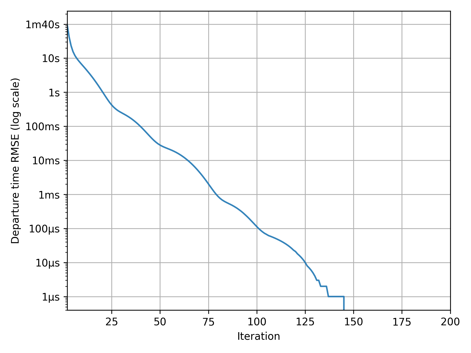
For the bottleneck simulation, you can focus on these graphs:

• convergence_tour_departure_time.png shows by how much departure times vary over iterations;
• convergence_simulated_road_travel_times.png shows by how much the simulated travel-time function differs from the expected travel-time function over iterations.

If your graphs match the examples below, with the indicator consistently at zero in the final iterations, the simulation has perfectly converged and results are reliable for analysis.

Note

At each iteration of METROPOLIS2, all agents choose their preferred departure time, across the entire possible departure-time period, based on the current expected travel-time function. If the simulated travel-time function matches the expected travel-time function, it means that agents made optimal choices: they accurately anticipated travel conditions and have no reason to change their departure time. Therefore, when departure times and travel times are unchanged between iterations, the simulation has effectively reached an equilibrium.

Tip

In this example, the simulation achieves perfect convergence. However, in more complex scenarios, perfect convergence may not always be attainable. Instead, ensure that the convergence indicators remain consistently low in the final iterations. This suggests that the simulation approximate an equilibrium, even if minor fluctuations persist. Such level of stability is often sufficient for meaningful analysis.

Results

Pymetropolis generates a variety of output files that you can use to analyze the simulation results. The most relevant files for the bottleneck simulation are:

• results/iteration_results.parquet gives aggregate results across all iterations;
• results/trip_results.parquet gives trip-level results, including departure times, arrival times, utilities.

Feel free to explore these files to generate your own tables and graphs.

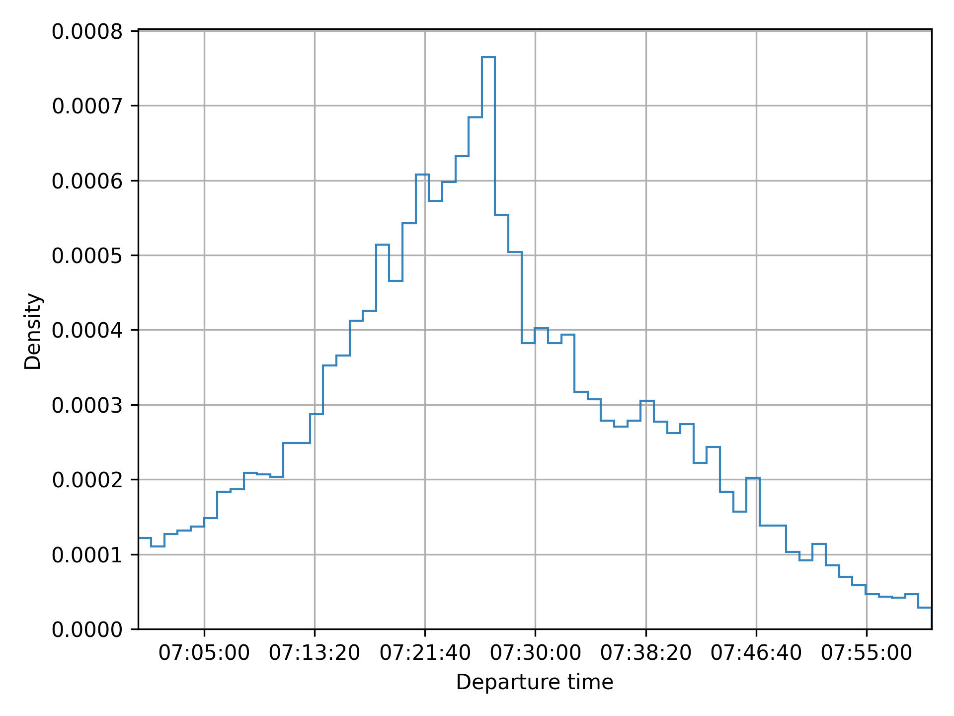
Pymetropolis also produces graphs to visualize key aspects of the simulation:

• results/graphs/trip_departure_time_distribution.png for the distribution of departure times;
• results/graphs/network_congestion_function_expected.png for the congestion function on the road.

For additional graphs and a comparison with analytical results, refer to Javaudin and de Palma (2024).

Extensions

Elastic demand

A simple way to extend the bottleneck model is to incorporate elastic demand by giving agents an alternative to traveling by car. This alternative could represent options like using public transit or choosing not to travel at all.

In Pymetropolis, you can model such an alternative using the "outside_option" mode. This mode provides a constant cost (or utility) alternative to the agents, without modeling departure times or travel times.

The modes.outside_option.constant parameter defines the constant cost associated to the outside option. Based on the previous simulation results, where agents’ surplus is around 7.25, you can set the outside option’s utility to 5 (i.e., its cost to -5) to ensure it remains less attractive than driving.

[modes.outside_option]
constant = -5

Caution

The [modes.outside_option] table must be nested within the [modes] section. If you are unsure about the syntax, refer to the TOML documentation or the complete configuration example below for guidance.

Adding the outside option introduces a new decision for agents: choosing between driving or not. You need to specify how agents choose between these two options, using the mode_choice.model parameter.

A standard approach is to use a Logit model, which allows agents to make probabilistic choices based on the utility of each option. Configure this by updating the [mode_choice] table in your configuration, setting mode_choice.model to "Logit".

[mode_choice]
modes = ["car_driver", "outside_option"]
model = "Logit"
mu = 1

The mode_choice.mu parameter controls the level of randomness in the choice: smaller values make agents more likely to choose the utility-maximizing option; larger values introduce more randomness in their decision. Also observe that you need to include "outside_option" in the list of modes available to the agents.

Distributed parameters

So far, the simulated agents were identical: they shared the same origin, destination, value of time, schedule-delay penalties, and desired arrival time. Crucially, some form of heterogeneity was introduced through the Continous Logit model (for departure-time choice) and the Logit model (for mode choice). This heterogeneity is essential to prevent all agents from choosing the same departure time, which would result in unrealistic congestion patterns.

You can introduce additional variability by defining preference parameters, such as modes.car_driver.alpha or departure_time.linear_schedule.beta, as distributions rather than fixed values. For example, to model the desired arrival time as a Normal distribution with a mean of 07:30:00 and a standard deviation of 10 minutes (600 seconds), you can use the following configuration.

tstar = { mean = 07:30:00, std = 600, distribution = "Normal" }

The same syntax can be applied to any preference parameter that supports distributions. For more details on the syntax and the available distributions, refer to the Parameters page.

Complete configuration

main_directory = "bottleneck-sim/"

random_seed = 123454321

[grid_network]
nb_rows = 1
nb_columns = 2
length = 1000
right_to_left = false

[road_network]
default_speed_limit = 120
capacities = 16_000

[node_od_matrix]
each = 10_000

[mode_choice]
modes = ["car_driver"]
# Uncomment to add the outside option alternative.
#modes = ["car_driver", "outside_option"]
#model = "Logit"
#mu = 1

[modes]
[modes.car_driver]
alpha = 10

# Uncomment to add the outside option alternative.
#[modes.outside_option]
#constant = -5

[departure_time_choice]
model = "ContinuousLogit"
mu = 1

[departure_time.linear_schedule]
beta = 5
gamma = 7
# Constant tstar over agents.
tstar = 07:30:00
# Normally distributed tstar over agents.
#tstar = { mean = 07:30:00, std = 600, distribution = "Normal" }

[simulation]
period = [07:00:00, 08:00:00]
recording_interval = 60
learning_factor = 0.1
nb_iterations = 200

[metropolis_core]
exec_path = "execs/metropolis_cli"

References

Arnott, R., de Palma, A., & Lindsey, R. (1990). Economics of a bottleneck. Journal of urban economics, 27(1), 111-130.

de Palma, A., Ben-Akiva, M., Lefevre, C., & Litinas, N. (1983). Stochastic equilibrium model of peak period traffic congestion. Transportation Science, 17(4), 430-453.

Javaudin, L., & de Palma, A. (2024). METROPOLIS2: Bridging theory and simulation in agent-based transport modeling. Technical report, THEMA, CY Cergy Paris Université.

Vickrey, W. S. (1969). Congestion theory and transport investment. The American economic review, 59(2), 251-260.