Circular City (Toy model)
Estimated time to complete: 2 hours
This case study presents a toy model designed to be both simple and feature-rich:
- Quick to run: Executes in just a few minutes.
- Concise configuration: Requires only a single TOML file (~100 lines).
- Comprehensive: Incorporates most of METROPOLIS2’s core features, including mode choice, departure-time choice, route choice, fuel consumption, spillback effects, and ridesharing.
The model simulates an imaginary circular city, featuring ring roads (circular roads) and radial roads (arterial roads).
This structure is inspired by the foundational work of de Palma, Kilani, and Lindsey (2005), though it is not an exact replication. Instead, it offers a modern adaptation tailored for METROPOLIS2.
Preparation
As for the Bottleneck case study, begin by creating a TOML configuration file
(e.g., config-circular-city.toml) in your preferred directory.
This file serves as the foundation for your simulation.
Start by defining the main_directory and
random_seed parameters in your configuration file.
The main_directory specifies where all simulation outputs will be saved, while the random_seed
ensures your results are reproducible.
# config-circular-city.toml
main_directory = "circular-city/"

random_seed = 123454321
Supply side
The Circular City model uses the CircularNetworkStep
to create a customizable road network composed of ring roads and radial roads.
The nb_radials parameter defines the
number of directions for radial roads:
nb_radials = 4: creates radial roads in the North, East, South, and West directions;nb_radials = 8: adds Northeast, Northwest, Southeast, and Southwest directions;nb_radials = n: n roads are automatically generated starting from the East direction and are evenly spaced around the circle.
Parameter nb_rings controls the number of
concentric rings in the city and parameter
radius defines the distance between rings
(in meters).
If radius is a single value, for example radius = 2000, each ring is space 2 km apart from the
city center.
If radius is a list, for example radius = [1000, 1500] (with nb_rings = 2), the first ring is
1 km from the center and the second is 1.5 km from the center (500 m apart).
Nodes are automatically created at the intersection of each ring and radial road.
For more details, including how node and edge ids are generated, refer to the
CircularNetworkStep documentation.
For the same topological network as in de Palma et al. (2005), use the following configuration. Feel free to tweak it to your liking!
[circular_network]
nb_radials = 8
nb_rings = 4
radius = 4000
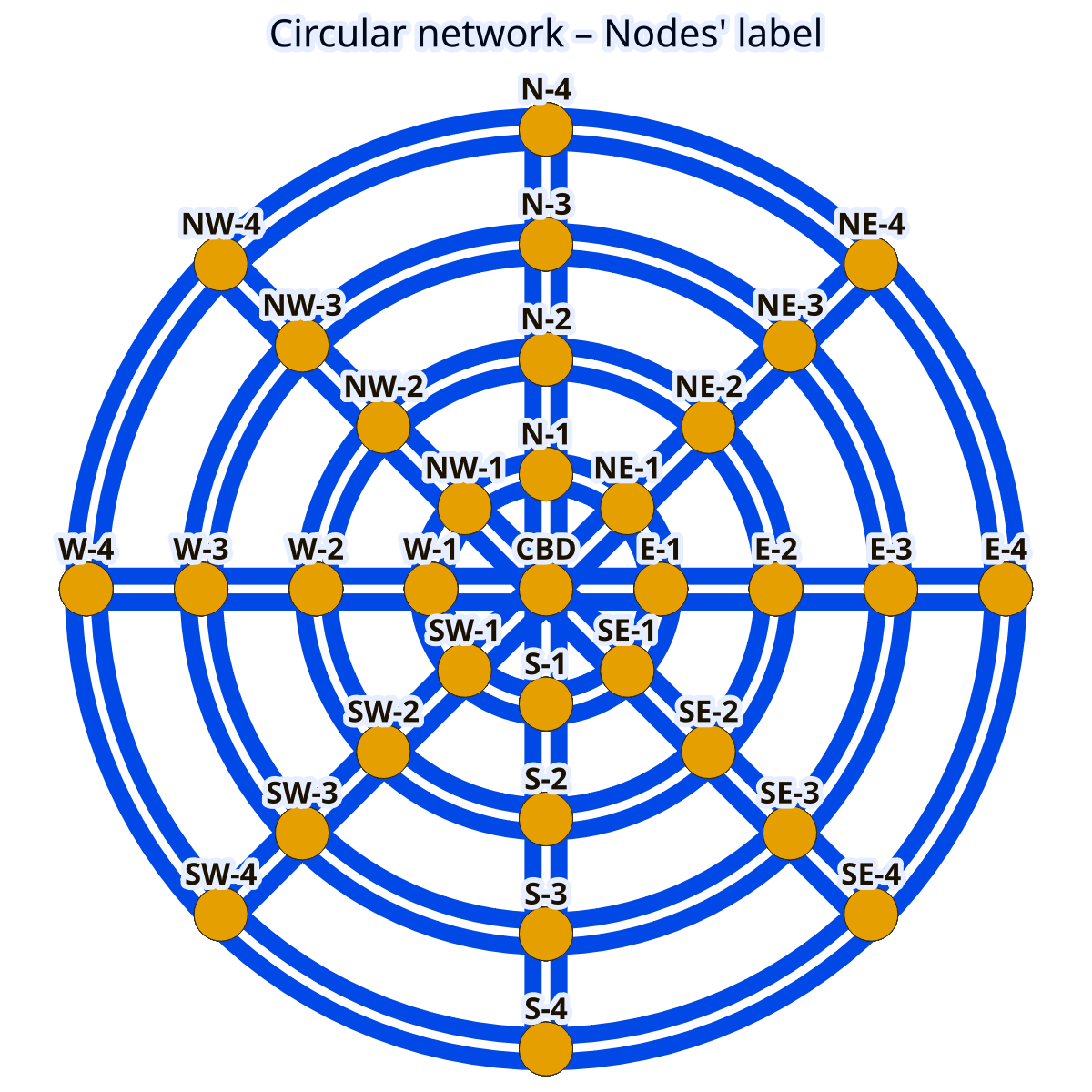
Figure 1. Circular network with node labels.
File used: edges_raw.geo.parquet
Tip
If you are more into American-style cities, consider creating a grid network instead.
To finalize the Circular City network configuration, you need to define the speed limits, number of
lanes and bottleneck capacities.
This is done using
PostprocessRoadNetworkStep and
ExogenousCapacitiesStep, similar to the
Bottleneck case study.
The key parameters are:
road_network.default_speed_limitsets the speed limit (in km/h);road_network.default_nb_lanesdefines the number of lanes (in one direction);road_network.capacitiesspecifies the bottleneck capacity (in vehicles per hour per lane).

Figure 2. Circular network with edges’ road types.
Edges with the same color share the same road type.
File used: edges_raw.geo.parquet
The values can be specified per road type (see map) by providing a TOML table with the road-type labels as keys. To replicate the values from de Palma et al. (2005), use the following configuration.
[road_network]
[road_network.default_speed_limit]
"Radial 1" = 50
"Radial 2" = 50
"Radial 3" = 50
"Radial 4" = 50
"Ring 1" = 50
"Ring 2" = 70
"Ring 3" = 70
"Ring 4" = 70

[road_network.default_nb_lanes]
"Radial 1" = 2
"Radial 2" = 2
"Radial 3" = 2
"Radial 4" = 2
"Ring 1" = 1
"Ring 2" = 1
"Ring 3" = 1
"Ring 4" = 1

[road_network.capacities]
"Radial 1" = 1500
"Radial 2" = 2000
"Radial 3" = 2000
"Radial 4" = 2000
"Ring 1" = 2000
"Ring 2" = 2000
"Ring 3" = 2000
"Ring 4" = 2000
Demand side
To simulate trips in the Circular City model, you can use an origin-destination matrix, where road-network nodes serve as origins and destinations.
In real-world scenarios, the number of trips between two nodes typically decreases with distance.
The GravityODMatrixStep models this effect by
assuming that the number of trips between nodes decays exponentially with distance.
The key parameters for this step are defined below.
trips_per_nodedefines the total number of trips originating from each node.exponential_decaycontrols how quickly the number of trips decreases with distance. Withexponential_decay = 0, trips originating from a node are uniformly distributed across all destinations. With higher values, more trips are concentrated toward closer destinations.
[gravity_od_matrix]
trips_per_node = 8000
exponential_decay = 0.07

Figure 3. Flows originating from node “NE-2”.
Files used: road_origin_destination_matrix.geo.parquet,
edges_raw.geo.parquet
Tip
If you want different number of trips originating from each node, you can define
trips_per_nodeas a distribution. For example:
trips_per_node = { mean = 8000, std = 1000, distribution = "Normal" }
Tip
For full control over trip generation, you can create your own origin-destination matrix and use it with the
CustomODMatrixStep.
To align with de Palma et al. (2005), you can configure agents to choose between car and public transit using a Logit model. This setup allows agents to make probabilistic choices based on the utility of each mode.
[mode_choice]
modes = ["car_driver", "public_transit"]
model = "Logit"
mu = 1
The parameters are defined as follow.
modeslists the available travel modes.modeluses the Logit model for mode choice.mucontrols the randomness in mode select. Lower values means that agents are more likely to choose the maximum-utility mode.
Tip
For more advanced scenarios, you can include ridesharing as an additional mode. This extension is explored further in the Extensions section.
Preferences for each mode are defined in the modes.* tables.
Each mode includes two parameters.
alpharepresents the value of time (in euros per hour).constantrepresents a fixed cost associated with choosing the mode.
[modes]
[modes.car_driver]
constant = 0
alpha = 10

[modes.public_transit]
constant = 2.0
alpha = 15.0
road_network_speed = 40
The parameter
road_network_speed simplifies
public-transit travel time calculation by assuming a constant speed on the road network, avoiding
the need to define a separate public-transit network.
A value of 40 km/h matches the assumption from de Palma et al. (2005).
As in the Bottleneck case study, you can include schedule-delay penalties in the
utility function using the departure_time.linear_schedule table.
These penalties influence agents’ departure-time choice based on their desired arrival time.
betadefines the penalty for early arrivals (in euros per hour).gammadefines the penalty for late arrivals (in euros per hour).tstarrepresent the desired arrival time at destination, specified inHH:MM:SSformat.
[departure_time.linear_schedule]
beta = 6
gamma = 25
tstar = { mean = 08:00:00, std = 1800, distribution = "Uniform" }
This configuration means that agents have a desired arrival time uniformly distributed between
07:30:00 and 08:30:00.
Late arrivals incur a higher penalty (25 euros per hour) compared to early arrivals (6 euros per
hour).
To model how agents choose their departure time, it is recommended using the Continuous Logit model, which aligns with the approach in de Palma et al. (2005).
Set departure_time_choice.model
to "ContinuousLogit" and use
departure_time_choice.mu to control
the randomness in agents’ choices: smaller values make agents choose departure times closer
to the utility-maximizing value; larger values introduce more randomness in their choice.
[departure_time_choice]
model = "ContinuousLogit"
mu = 1
Simulation
Before running the simulation, configure the final parameters in the simulation table.
[simulation]
period = [06:00:00, 10:00:00]
recording_interval = 300
learning_factor = 0.005
nb_iterations = 200
The simulation.period parameter defines
the time window of the simulation, specified as a list of start and end times.
This period constrains when agents can depart.
For this simulation, focused on the morning peak period (with desired arrival times between 07:30 and 08:30), a period from 6 a.m. to 10 a.m. provides a sufficiently wide window for all agents to depart and reach their destinations.
Tip
If you notice a peak of departures at the very start or end of the simulation period, it may indicate that the period is too narrow. Extend the window to allow agents to choose departure times that align better with their desired arrival times.
The simulation.recording_interval
parameter controls the time between breakpoints in the piecewise linear functions used to store
travel times.
A value of 300 seconds (5 minutes) offers a good balance between simulation speed and accuracy in
travel-time functions.
To ensure the simulation converges satisfactorily, two key parameters are defined.
simulation.learning_factorcontrols how quickly agents learns about travel times. A value of 0.005 is recommended for this simulation.simulation.nb_iterationsdetermines the number of iterations the simulation runs. A value of 200 is typically sufficient.
Tip
For simulations with higher congestion, consider decreasing the learning factor or increasing the number of iterations to improve the convergence quality.
For more details on simulation convergence, refer to the relevant page.
Before running your simulation, ensure you have downloaded the last version of
Metropolis-Core and configured the
metropolis_core.exec_path parameter to
point to the metropolis_cli executable.
By convention, the executable is typically placed in an execs/ directory within the directory
where Pymetropolis is executed.
[metropolis_core]
exec_path = "execs/metropolis_cli"
Running
Once your configuration file is ready, you can execute Pymetropolis directly from the terminal.
Simply run the pymetropolis command, specifying the path to your configuration file as an
argument.
Optionally, before running the full simulation, you can check what Pymetropolis is planning to do by
using the --dry-run option.
This will check for typos or issues and display the list of steps that will be executed:
pymetropolis config-circular-city.toml --dry-run
If there everything is correctly configured, you should see an output similar to this.
1. WriteMetroParametersStep
2. CircularNetworkStep
3. PostprocessRoadNetworkStep
4. AllRoadDistancesStep
5. ExogenousCapacitiesStep
6. EdgesFreeFlowTravelTimesStep
7. AllFreeFlowTravelTimesStep
8. GravityODMatrixStep
9. CarFreeFlowDistancesStep
10. CarShortestDistancesStep
11. GenericPopulationStep
12. WriteMetroEdgesStep
13. WriteMetroVehicleTypesStep
14. CarDriverPreferencesStep
15. PublicTransitPreferencesStep
16. PublicTransitTravelTimesFromRoadDistancesStep
17. RoadODMatrixStep
18. LinearScheduleStep
19. HomogeneousTstarStep
20. WriteMetroTripsStep
21. UniformDrawsStep
22. WriteMetroAgentsStep
23. WriteMetroAlternativesStep
24. RunSimulationStep
25. IterationResultsStep
26. ConvergencePlotStep
27. RoadNetworkCongestionFunctionPlotsStep
28. TripResultsStep
29. TripDepartureTimeDistributionStep
If the list of steps looks correct, you can proceed with the actual simulation by removing the
--dry-run option.
pymetropolis config-circular-city.toml
The simulation should complete in about 20 minutes.
Convergence
Before diving into the results, the first step is to verify whether the simulation has converged satisfactorily. If the convergence is poor, further analysis may not be meaningful, and you may need to adjust the number of iterations or the learning factor (See Simulation convergence).
Pymetropolis automatically generates convergence graphs in the results/graphs/ directory (located
within the main_directory you specified).
These graphs are prefixed with convergence_ and fall into two main categories.
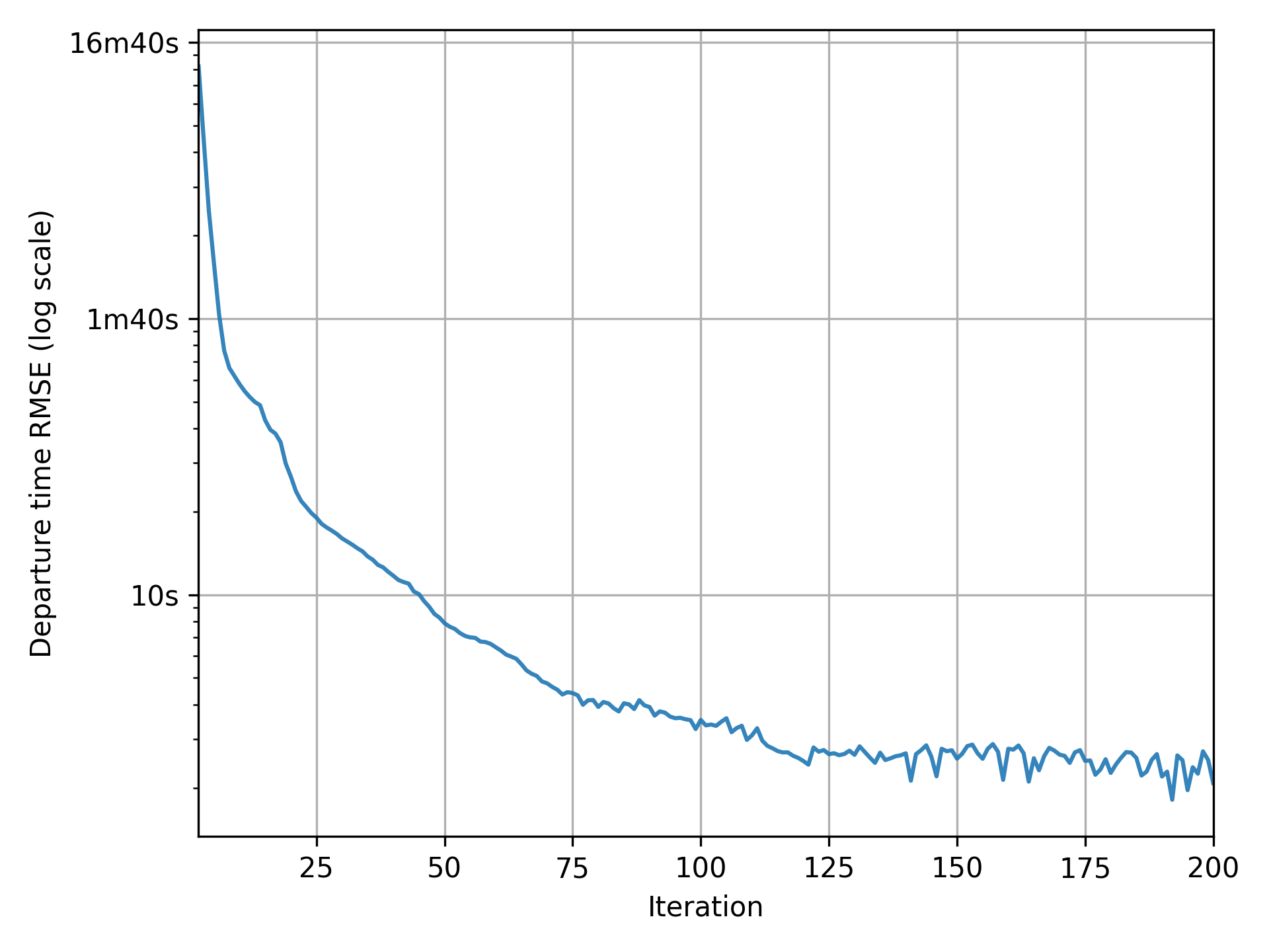
- Graphs with an indicator representing a change from one iteration to another.
The indicator should be close to zero in the final iterations.
Example graphs:
convergence_tour_departure_time.png: shifts in departure times,convergence_route_length_diff.png: shifts in route selected,convergence_simulated_road_travel_times.png: changes in road-level travel times.
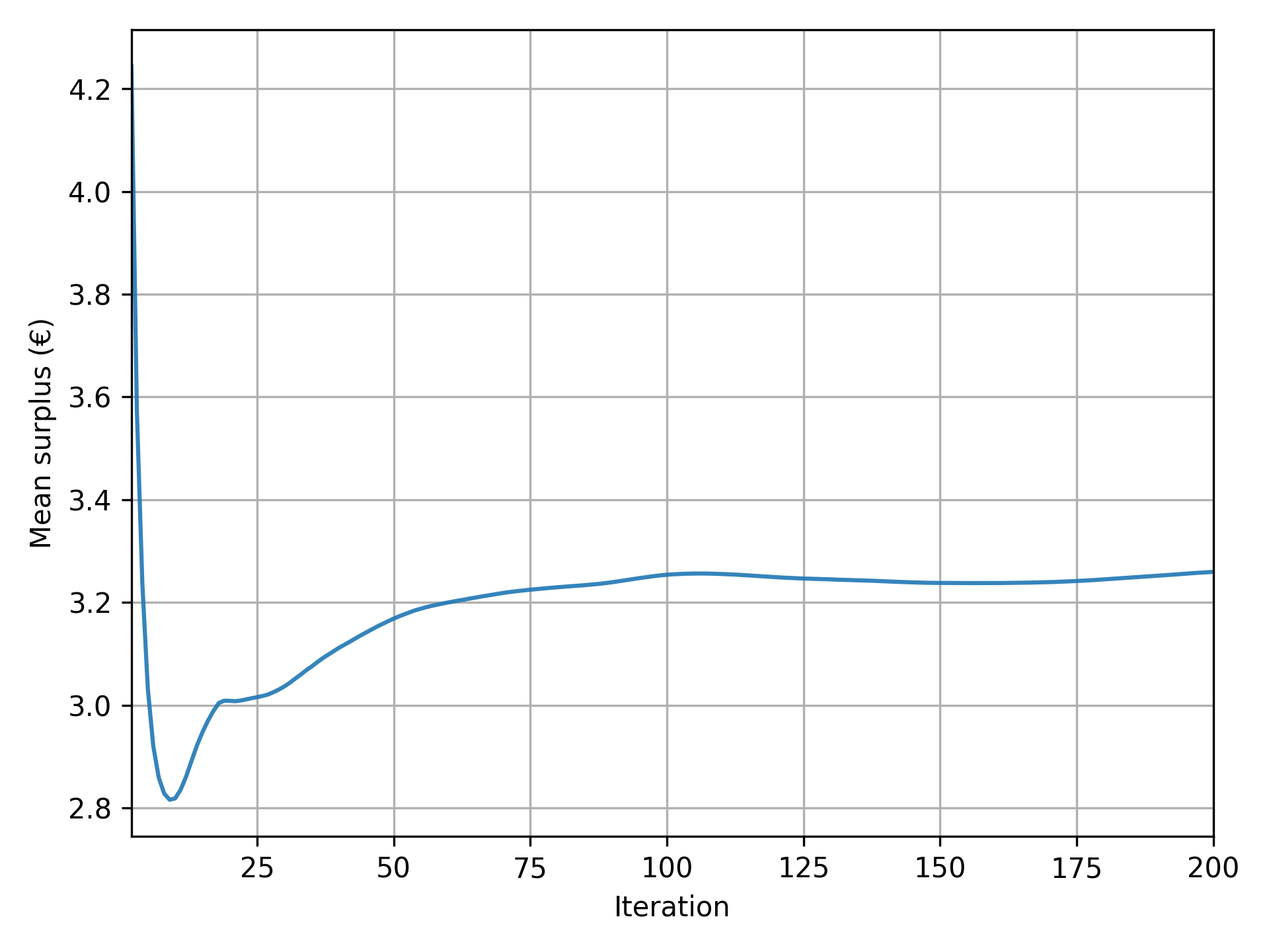
- Graphs with an indicator representing an aggregate measure.
The indicator should stabilize to an equilibrium value in the final iterations.
Example graphs:
convergence_mean_surplus.png: mean surplus,convergence_road_trips_share.png: share of road trips.
Results
Pymetropolis generates a variety of output files that you can use to analyze the simulation results. Some of the most relevant files are:
results/iteration_results.parquetgives aggregate results across all iterations;results/trip_results.parquetgives trip-level results, including departure times, arrival times, utilities.
Feel free to explore these files to generate your own tables and graphs.
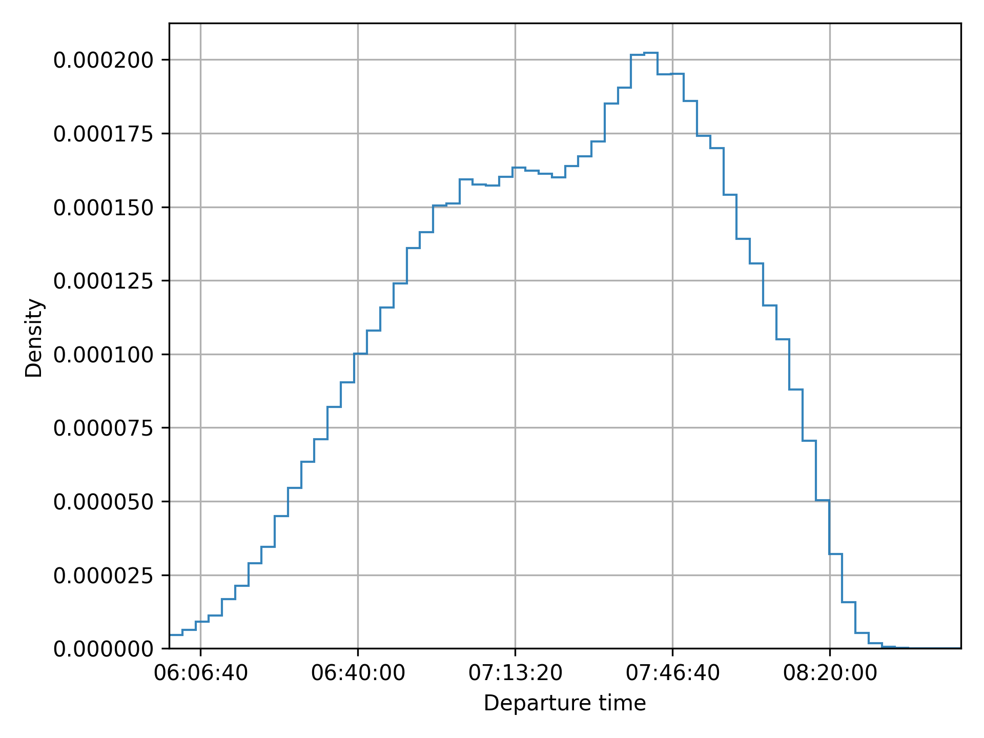
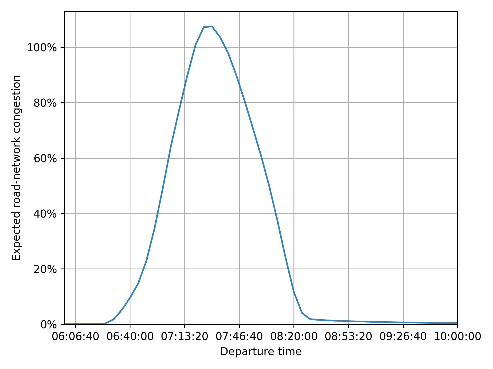
Pymetropolis also produces graphs to visualize key aspects of the simulation:
results/graphs/trip_departure_time_distribution.pngfor the distribution of departure times;results/graphs/network_congestion_function_expected.pngfor the congestion function on the road.
Complete configuration
main_directory = "circular-city/"

random_seed = 123454321

[circular_network]
nb_radials = 8
nb_rings = 4
radius = 4000

[road_network]
[road_network.default_speed_limit]
"Radial 1" = 50
"Radial 2" = 70
"Radial 3" = 70
"Radial 4" = 70
"Ring 1" = 50
"Ring 2" = 50
"Ring 3" = 50
"Ring 4" = 50

[road_network.default_nb_lanes]
"Radial 1" = 2
"Radial 2" = 2
"Radial 3" = 2
"Radial 4" = 2
"Ring 1" = 1
"Ring 2" = 1
"Ring 3" = 1
"Ring 4" = 1

[road_network.capacities]
"Radial 1" = 1500
"Radial 2" = 2000
"Radial 3" = 2000
"Radial 4" = 2000
"Ring 1" = 2000
"Ring 2" = 2000
"Ring 3" = 2000
"Ring 4" = 2000

[gravity_od_matrix]
exponential_decay = 0.07
trips_per_node = 8000

[mode_choice]
modes = ["car_driver", "public_transit"]
model = "Logit"
mu = 1

[modes]
[modes.car_driver]
constant = 0
alpha = 10

[modes.public_transit]
constant = 2
alpha = 15
road_network_speed = 40

[departure_time_choice]
model = "ContinuousLogit"
mu = 1

[departure_time.linear_schedule]
beta = 6
gamma = 25
tstar = { mean = 08:00:00, std = 1800, distribution = "Uniform" }

[simulation]
period = [06:00:00, 10:00:00]
recording_interval = 300
learning_factor = 0.005
nb_iterations = 200

[metropolis_core]
exec_path = "execs/metropolis_cli"
Extensions
Introducing ridesharing
In the current setup, agents traveling by car are assumed to be driving alone, with each agent generating congestion equivalent to a single car. However, in reality, people with similar origins and destinations often share rides to save on costs like fuel.
METROPOLIS2 proposes the "car_ridesharing" mode to model ridesharing.
This mode represents agents traveling by car with others, without distinguishing between drivers
and passengers.
To include this mode as an option for the agents, update the
mode_choice.modes parameter.
[mode_choice]
modes = ["car_driver", "car_ridesharing", "public_transit"]
Note
The
"car_ridesharing"mode is a basic representation of ridesharing in METROPOLIS2:
- It does not explicitly model the matching between drivers and passengers.
- It does not guarantee that agents choosing ridesharing have a compatible partner with the same origin, destination, and departure time.
- It does not account for detours drivers might take to pick up or drop off passengers.
For advanced ridesharing modeling in METROPOLIS2, including matching, refer to Ghoslya et al. (2025).
You can define preferences for the "car_ridesharing" mode different from the ones for
"car_driver".
constantrepresents the fixed cost of ridesharing (e.g., difficulty finding a match, detours, waiting time).alpharepresents the value of time (which can be different from car alone due to inconvenience).
[modes.car_ridesharing]
constant = 2.0
alpha = 11.0
Since ridesharing involves multiple persons per car, the congestion generated must be adjusted. METROPOLIS2 simulates one car per ridesharing agent, but you can modify the Passenger Car Equivalent (PCE) and headway to reflect the reduced congestion impact of shared rides.
- If ridesharing agents travel in pairs, PCE and headway must be divided by 2.
- If they travel in groups of three, PCE and headway must be divided by 3.
- In general, if the average number of passengers per ridesharing car is n, PCE and headway must be divided by 1 + n.
The average number of passengers is controlled by the
vehicle_types.car.ridesharing_passenger_count
parameter.
For France, this value is approximately 1.2.
[vehicle_types]
[vehicle_types.car]
ridesharing_passenger_count = 1.2
Tip
You can also use the
"car_ridesharing"mode as a complete substitute for"car_driver"if you want to model ridesharing without distinguishing between solo and shared trips. In this case, you need to assume the same constant cost and value of time for all car trips. Additionally,ridesharing_passenger_countmust be set to the average number of passengers per car (including solo drivers). For France, this value is around 0.4 (or lower during peak hours).However, this approach is not adapted when you want to model different preferences for solo and shared trips and when you want to simulate HOV lanes.

Figure 4. Mode shares with the "car_ridesharing" option.
Adding fuel costs to car trips
In the current setup, ridesharing offers no clear individual benefit in the model:
- Both the constant cost and the value of time are larger than for car alone.
- Travel times are identical for solo and shared trips.
The only reason some agents choose "car_ridesharing" is due to the Logit model’s randomness, which
introduces variability in mode choice.
In reality, ridesharing is attractive because it allows sharing costs (e.g., fuel, tolls) among participants. METROPOLIS2 can model fuel costs using two parameters.
fuel.consumption_factorrepresents the fuel consumption rate for car trips, in liters per kilometer. A value of 0.08 equals a consumption of 8 liters per 100 km.fuel.pricedefines the price per liter of fuel, in euros.
[fuel]
consumption_factor = 0.08
price = 1.8
With this configuration, fuel cost are included in the utility function for both "car_driver" and
"car_ridesharing".
However, for "car_ridesharing", the fuel cost is divided by the ridesharing_passenger_count,
which can make ridesharing more attractive than driving alone.
Caution
METROPOLIS2 currently does not compute fuel consumption dynamically based on the selected route during each iteration. Instead, it uses pre-simulation free-flow consumption.
When fuel costs are included, the model shows an increase in both ridesharing and public-transit use.

Figure 5. Mode shares when including fuel costs.
Enhancing ridesharing with HOV lanes
High-Occupancy Vehicle (HOV) lanes are an effective way to make ridesharing more attractive. These lanes are restricted to cars with at least two passengers (including the driver). If they are less congested than regular lanes, they can reduce travel times for ridesharing user compared to solo drivers.
HOV lanes are defined using the
road_network.hov_lanes parameter.
This parameter works similarly to road_network.nb_lanes: you can specify a single
value (applied to all edges) or you can use a table to define HOV lanes for specific road types.
[road_network.hov_lanes]
"Ring 1" = 1
"Ring 2" = 1
In his example, edges with road types "Ring 1" and "Ring 2" have one HOV lane, while, for other
road types, the default value (no HOV lane) is used.
Caution
The
road_network.hov_lanesdoes not add extra lanes to edges. Instead, it reserves lanes from the total defined byroad_network.nb_lanes. An edge cannot have more HOV lanes than its total lanes (hov_lanes ≤ nb_lanes).You can create edges with only HOV lanes (
nb_lanes = hov_lanes), effectively banning solo drivers from those edges. However, ensure that solo drivers can still reach their destination via alternative routes.
Tip
Both
road_network.nb_lanesandroad_network.hov_lanessupport non-integer values. For example, you can sethov_lanes = 0.5to model HOV lanes in a “continuous” way.
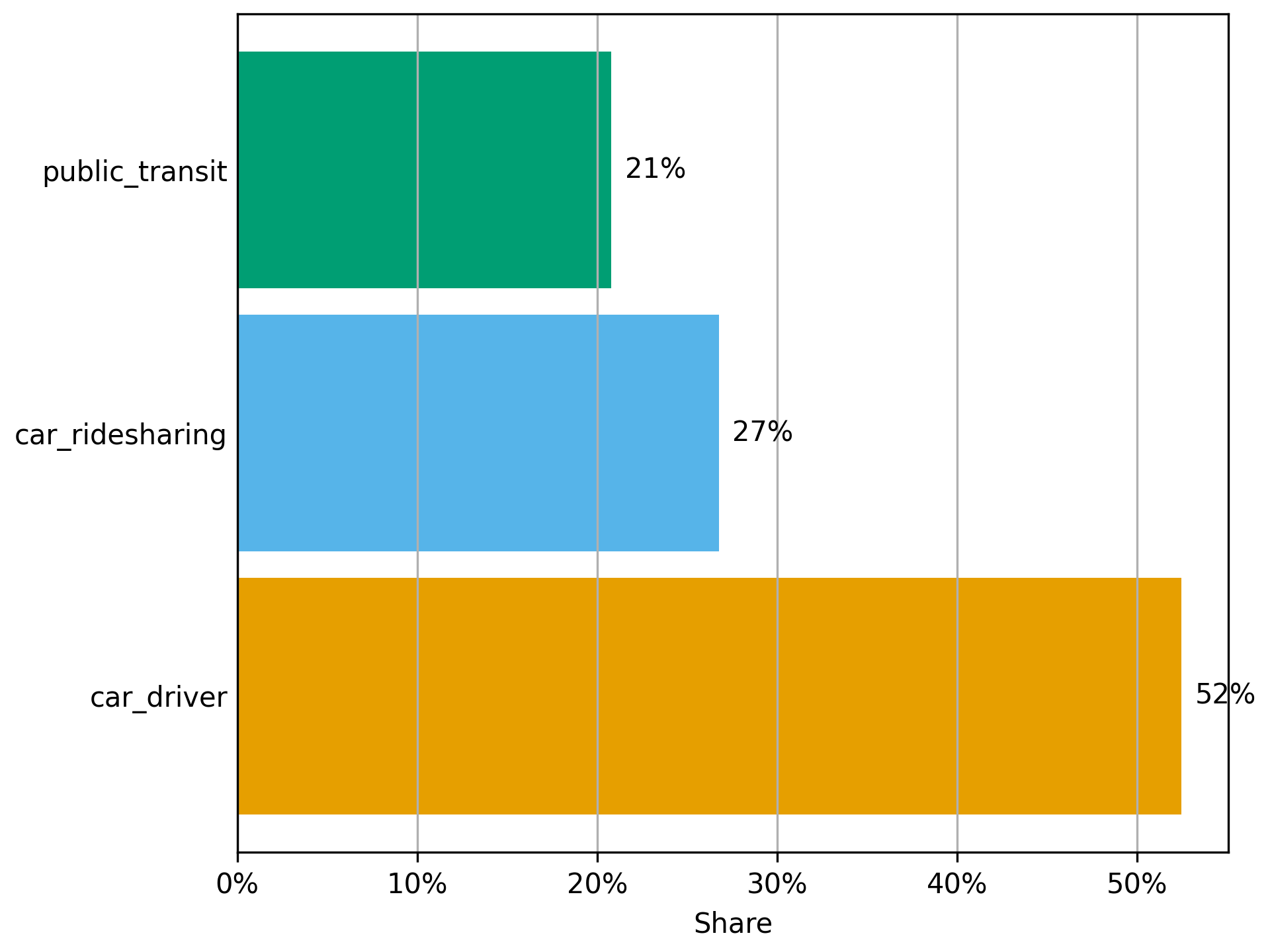
Figure 6. Mode shares with HOV lanes.
Matching constant
Coming soon.
Nested Logit for mode choice
Coming soon-ish.
Complete configuration with ridesharing
main_directory = "circular-city-ridesharing/"

random_seed = 123454321

[circular_network]
nb_radials = 8
nb_rings = 4
radius = 4000

[road_network]
[road_network.default_speed_limit]
"Radial 1" = 50
"Radial 2" = 50
"Radial 3" = 50
"Radial 4" = 50
"Ring 1" = 50
"Ring 2" = 70
"Ring 3" = 70
"Ring 4" = 70

[road_network.default_nb_lanes]
"Radial 1" = 1
"Radial 2" = 1
"Radial 3" = 1
"Radial 4" = 1
"Ring 1" = 2
"Ring 2" = 2
"Ring 3" = 2
"Ring 4" = 2

[road_network.capacities]
"Radial 1" = 1500
"Radial 2" = 2000
"Radial 3" = 2000
"Radial 4" = 2000
"Ring 1" = 2000
"Ring 2" = 2000
"Ring 3" = 2000
"Ring 4" = 2000

[road_network.hov_lanes]
"Ring 1" = 1
"Ring 2" = 1

[gravity_od_matrix]
exponential_decay = 0.07
trips_per_node = 8000

[mode_choice]
modes = ["car_driver", "car_ridesharing", "public_transit"]
model = "Logit"
mu = 1.0

[modes]
[modes.car_driver]
constant = 0.0
alpha = 10.0

[modes.car_ridesharing]
constant = 2.0
alpha = 11.0

[modes.public_transit]
constant = 2.0
alpha = 15.0
road_network_speed = 40

[departure_time_choice]
model = "ContinuousLogit"
mu = 1.0

[departure_time.linear_schedule]
beta = 6.0
gamma = 25.0
tstar = { mean = 08:00:00, std = 1800, distribution = "Uniform" }

[vehicle_types]
[vehicle_types.car]
ridesharing_passenger_count = 1.2

[fuel]
consumption_factor = 0.08
price = 1.8

[simulation]
period = [06:00:00, 10:00:00]
recording_interval = 300
learning_factor = 0.005
nb_iterations = 200

[metropolis_core]
exec_path = "execs/metropolis_cli"
References
de Palma, A., Kilani, M., & Lindsey, R. (2005). Congestion pricing on a road network: A study using the dynamic equilibrium simulator METROPOLIS. Transportation Research Part A: Policy and Practice, 39(7-9), 588-611.
Ghoslya, S., Javaudin, L., Palma, A. D., & Delle Site, P. (2025). Ride-sharing, congestion, departure-time and mode choices: A social optimum perspective. Available at SSRN 5465467.